
A practical guide to exploring published breast cancer data - from Cell Ranger™ output count matrices through quality control, clustering and annotation, to publishable figures in TrailmakerⓇ Insights.
Are you working with single cell RNA-sequencing data generated using 10x Genomics Chromium and want to explore it without writing code?
Trailmaker supports downstream analysis and visualization of supported 10x Chromium gene expression data. The tool is free for all academic researchers. You need a Trailmaker account, but academic researchers do not need to purchase Parse Biosciences products to use it. (Note that industry scientists should contact Parse Biosciences to discuss Trailmaker access.)
In this tutorial, we’ll use publicly available mouse breast cancer data to explore the steps from uploading count matrices to exploring cell populations and creating figures.
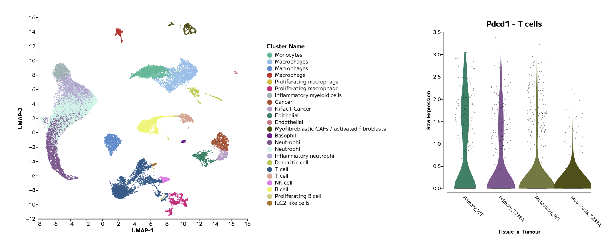
Figure 1: An example annotated UMAP and violin plot, showing Pdcd1 gene expression in T cells across groups of interest, generated in Trailmaker.
What you’ll learn
In this tutorial, we’ll follow the essential steps in single cell RNA-seq data analysis. By following this tutorial, you’ll learn how to:
Upload per-sample gene expression count matrices
Assign samples to groups with metadata
Review sample quality control and filtering
Integrate samples together in a single analysis and control for batch effects
Inspect cell clusters and annotate cell types
Compare gene expression across cell populations to discover biological insights
Generate, customise and export figures
Our guiding question is: Which major cell populations are present in these breast tumours, and how can we explore their gene expression patterns in a user-friendly tool?

Figure 2: An example single cell RNA-sequencing data analysis workflow using Trailmaker.
How does 10x Chromium data analysis work?
After sequencing, software such as Cell Ranger processes the sequencing reads into cell-by-gene count matrices. These matrices record counts for genes across cell barcodes and provide the starting point for downstream analysis and data visualization.
The downstream analysis workflow is very similar across single cell RNA-seq technologies: sample quality is reviewed and poor quality barcodes filtered out, gene expression is normalised, multi-sample datasets are integrated to control for batch effects, cell types are annotated, clusters are explored, and differential gene expression and pathways are analysed.
Not only are these steps possible in a graphical interface with Trailmaker Insights, the sample quality control step within Trailmaker is tailored for the technology type, including specific optimizations for 10x Chromium data.
This tutorial starts with count matrices that have already been generated and shared publicly in a research paper. You will not need to process FASTQ files or run Cell Ranger to follow the example presented in this tutorial.
About the dataset
We’ll use data from Wang and colleagues’ study, “ENPP1 is an innate immune checkpoint of the anticancer cGAMP–STING pathway in breast cancer,” published in PNAS in 2023.
The researchers investigated how ENPP1 contributes to the tumour environment and anti-tumour immunity. Their single cell experiment profiled primary breast tumours and lungs containing metastases from mice implanted with engineered 4T1 breast-cancer cells.
The data were generated using 10x Chromium Next GEM Single Cell 3′ HT v3.1 and processed with Cell Ranger. The authors used the Biomage-hosted instance of Cellenics, which is now Trailmaker, for downstream analysis.
The experiment contains eight samples, as detailed in Table 1 below:
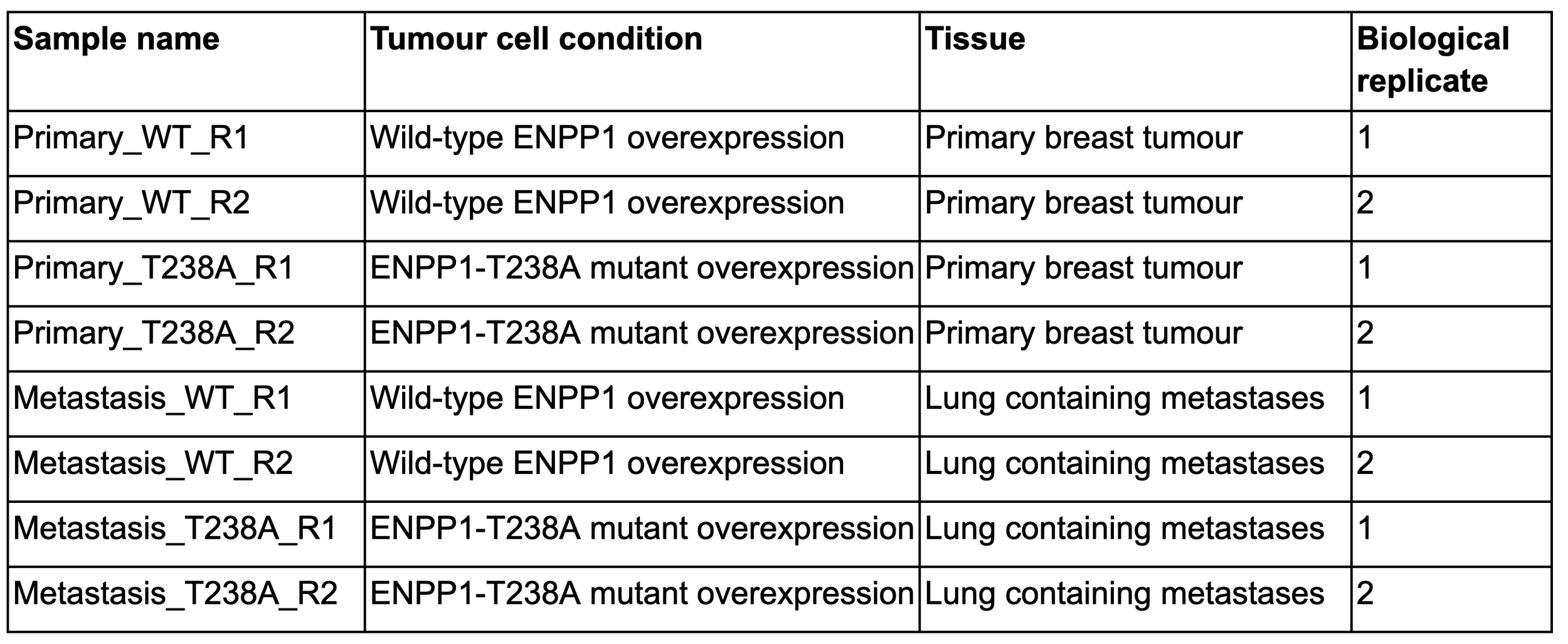
Table 1: Sample and metadata details for the tutorial dataset. The experimental setup was as follows: Enpp1-knockout 4T1 murine breast cancer cells overexpressing either WT ENPP1 (ENPP1WT-OE) or catalytically dead ENPP1 (ENPP1T238A-OE) were orthotopically implanted into WT mice, with the tissue sites of primary and metastatic tumours harvested for single cell RNA-seq analysis. Each mouse contributed a primary tumour sample and a lung sample, giving 8 tissue samples from 4 mice, with replicates illustrated in the final column.
1. Download the count matrices
Open the GEO dataset page for GSE233659. Under supplementary files, download GSE233659_RAW.tar (~260 MB) and extract the archive.
Despite “RAW” in its name, this archive contains processed count-matrix files, not raw sequencing reads.
Each sample has three associated files, which are located within the unzipped folder:
matrix.mtx.gz — gene-expression counts
features.tsv.gz — the corresponding gene or feature identifiers
barcodes.tsv.gz — the corresponding cell barcodes
The files will need to be organised within folders on your local drive before uploading to Trailmaker. Create a folder for each sample using the sample names in Table 1, above. Move the 3 associated files for each sample into the relevant sample folder. After doing this, you should have 8 folders (1 per sample), each containing 3 data files.
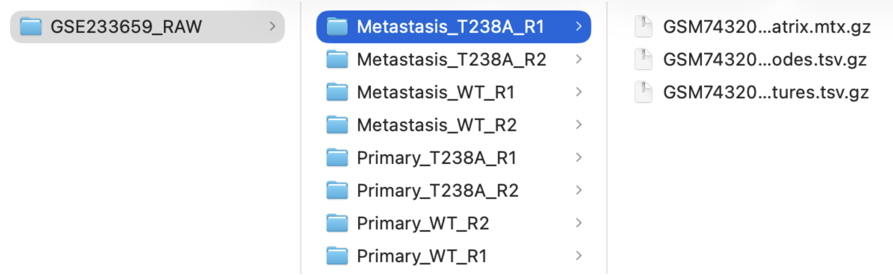
Figure 3: The recommended sample folder structure for data upload to Trailmaker.
Using your own data? Start with supported gene-expression count matrices or a supported gene-expression H5 file that are output from Cell Ranger. Trailmaker Insights accepts processed data from multiple technologies including 10x Chromium and Parse Evercode. Note that the Trailmaker Pipeline module processes Parse Evercode FASTQs only, and not 10x Chromium FASTQs.
See the Trailmaker upload requirements for further support to upload your own data.
2. Create an Insights project and upload your samples
Sign in to Trailmaker and open the Insights module.
Create a new project with a descriptive name, such as:
GSE233659 Breast tumour tutorial - Wang et al
Use the upload option appropriate for 10x Chromium count matrices (select ‘Add data’ -> select ‘10x Chromium’ in the Technology dropdown), then drag and drop your 8 sample folders to the upload box.
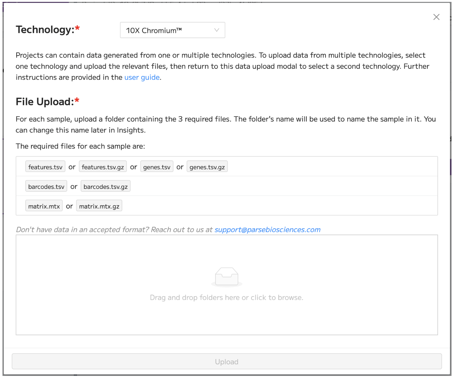
Figure 4: The data upload modal in Trailmaker Insights, showing the selection of ‘10x Chromium’ in the Technology dropdown menu.
The Insights setup walkthrough provides additional guidance on setting up a new project in Trailmaker.
3. Add experimental metadata
Once data upload is complete, add sample-level metadata within the Insights project details page in order to assign samples to groups. This is important as it allows the comparison and visualization of groups of interest.
For this tutorial, add the following sample-level metadata tracks:
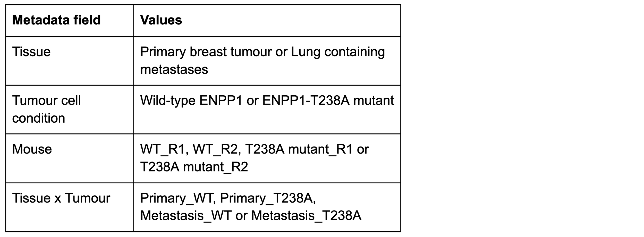
Table 2: Suggested sample-level metadata.
Clear metadata makes it easier to check whether patterns reflect individual samples, experimental conditions or cell populations.
After the addition of sample-level metadata, the Insights project details page view should look similar to Figure 5 below.
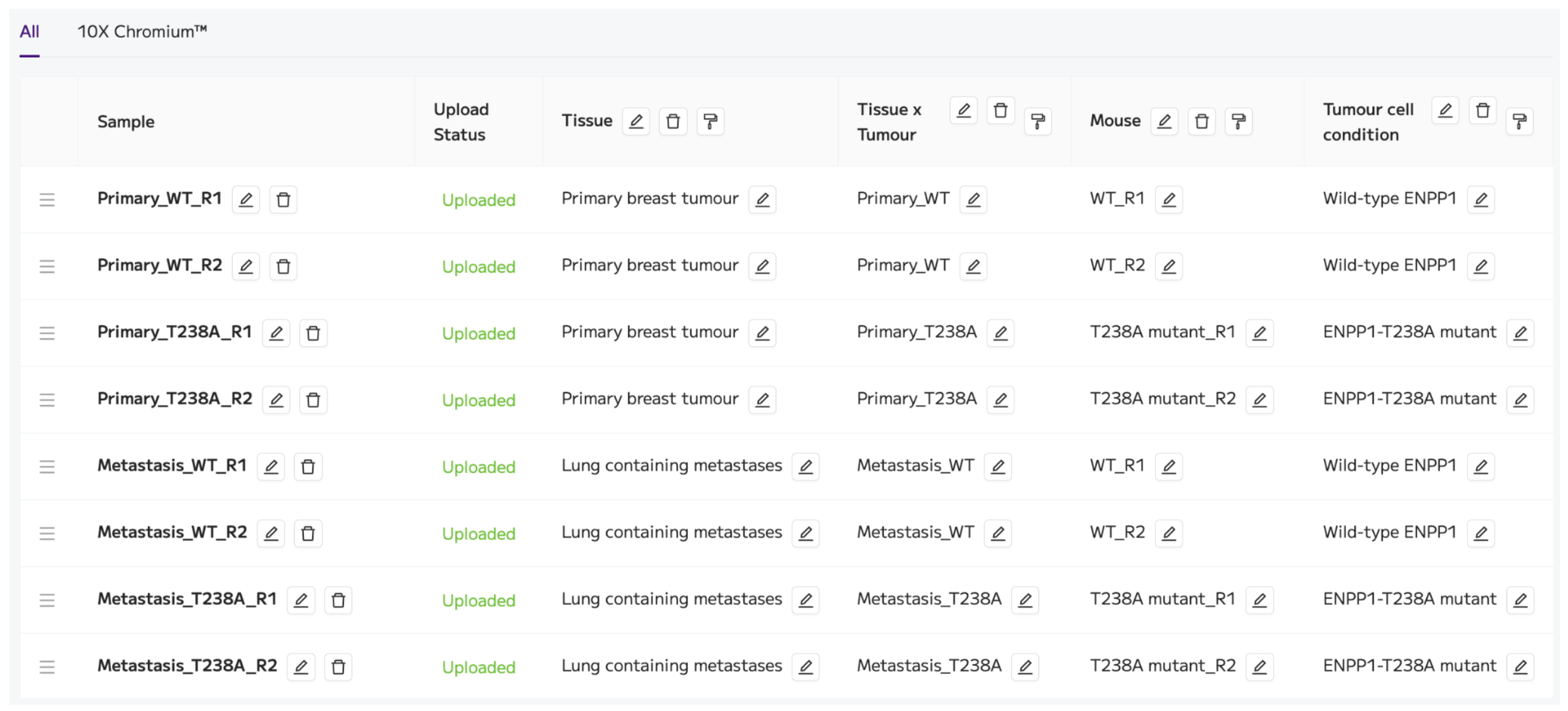
Figure 5: Trailmaker Insights project details page view containing the samples and metadata for the tutorial dataset.
The project is now ready to be processed using the ‘Process project’ button on the top right.
4. Review quality control
Once Data Processing has completed successfully, review the quality-control plots for each sample by carefully checking steps 1-5 of Data Processing (navigate through the steps using the dropdown menu or the arrows).
We uploaded the filtered count matrices that were output from Cell Ranger, which means that cell calling has already been performed in Cell Ranger. Within Trailmaker, steps 1-2 of Data Processing are disabled as cell calling has already been performed. We are performing cell quality filtering using Data Processing steps 3-5 to clean up the data in preparation for visualization.
Focus on what each metric tells you:
Counts per cell: Do some samples contain more/fewer barcodes with low signal?
Genes detected per cell: Are there cells with unusually low complexity?
Mitochondrial transcript fraction: Is there a population that may contain stressed or damaged cells?
Doublet scores: Are some profiles likely to represent more than one cell, such as doublets or multiplets?
Review the distributions alongside the automatic filtering threshold and the number of cells retained after filtering. Note any samples or metrics that are worthy of further investigation.
For example, the distribution of the mitochondrial content is quite different between the two ‘Primary_T238A’ replicates. This is reflected in the values of the automatic filtering threshold (17% for R1 and 11% for R2) and in the proportion of cells filtered out of these two samples at this step (10.4% for R1 and 7.5% for R2).
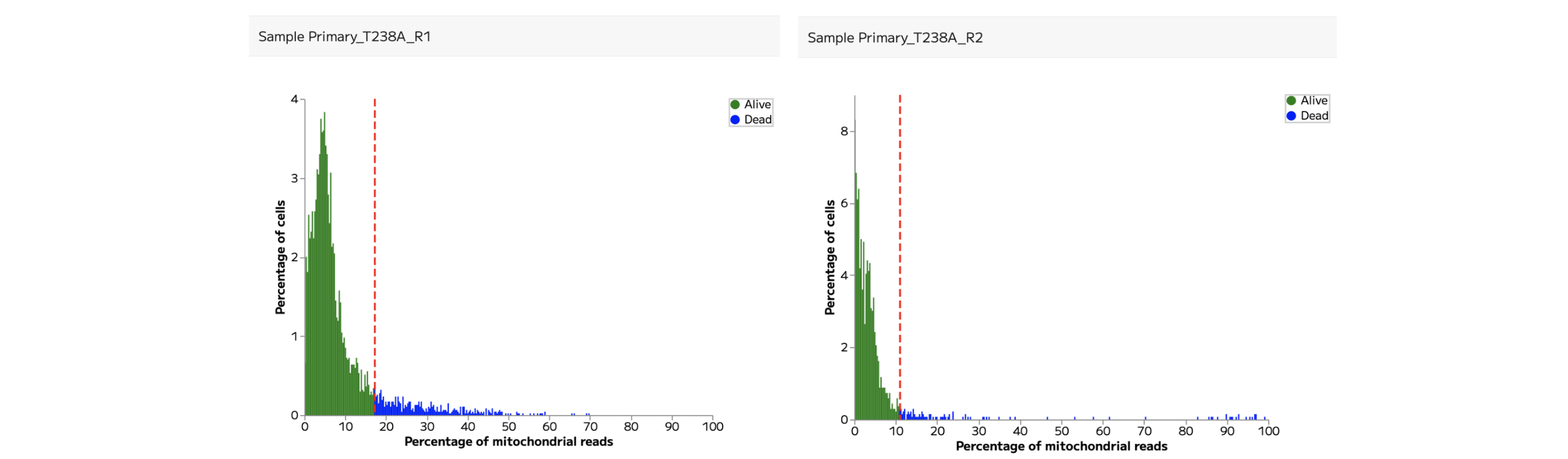
Figure 6: Mitochondrial content QC plots for the two ‘Primary_T238A’ replicates.
A threshold that works well for one sample or tissue may be inappropriate for another. Avoid adjusting filters simply to match a cell count or reproduce the appearance of a published plot. The aim is to retain informative cells using choices you can explain.
For the purposes of this tutorial, we’ll retain the automatic filtering for these two samples at the mitochondrial content filtering step.
5. Explore samples together and assess integration
Continue to integration, dimensionality reduction and clustering, which are shown in Data Processing steps 6 and 7.
Integration can help to remove artificial technical differences between samples, while retaining true biological differences. In Trailmaker, Harmony is the default integration method applied to the project. At this step the data are normalised using the logNormalization method.
Integration can be assessed using the UMAP and frequency plots in step 6.
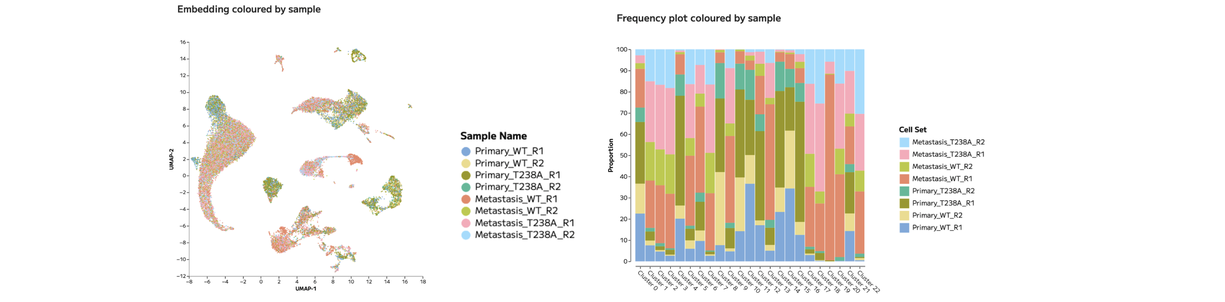
Figure 7: UMAP and Frequency plots coloured by sample allow the assessment of integration.
In the tutorial dataset, there are clear areas of the UMAP where cells from multiple samples overlap, while in other areas of the UMAP it appears that a few distinct samples dominate.
We should not assume that this effect reflects poorly integrated data. Instead, these separations may be the result of genuine biological differences between experimental groups. We’ll come back to this result later in the tutorial. For now, we’ll continue with the default integration settings.
The embedding and clustering parameters are set in Data Processing step 7. The default settings are: UMAP (t-SNE also available), Leiden clustering (Louvain also available), and clustering resolution of 0.8 (full manual control is available).

Figure 8: UMAP coloured by Leiden clusters, generated in Trailmaker using the default Data Processing settings.
We’ll now move on to the next module to annotate these clusters.
6. Annotate cell populations
In Trailmaker’s Data Exploration module, there are multiple ways to annotate cell populations. We have a dedicated article to support you through the annotation process: How to annotate cell types in Trailmaker.
There are three key features within Trailmaker that help with cell type annotation of single cell RNA-seq data.
A marker heatmap for the selected clustering method (in this case Leiden clusters) is shown at the bottom of the Data Exploration page.
The automatic annotation feature (“Annotate clusters”) can be selected within the Cell sets and Metadata tile of the Data Exploration page.
The Batch Differential Expression feature within the Plots and Tables module allows the download of marker gene lists for all Leiden clusters.
It is recommended to use broad labels first, followed by more detailed subtyping once the major populations are well supported. It is important to validate cell type identities using multiple known marker genes (ideally across multiple sources) rather than relying on a small number of genes.
For anyone who started at step 1 of this tutorial, we’ll start the annotation process by inspecting the annotation method reported in the published paper. In the supplementary information, a dot plot shows the marker genes for the labelled populations. We can use this dot plot together with the marker gene lists for the Leiden clusters to manually recreate the annotations from the paper using the ‘Custom cell sets’ feature in Trailmaker.
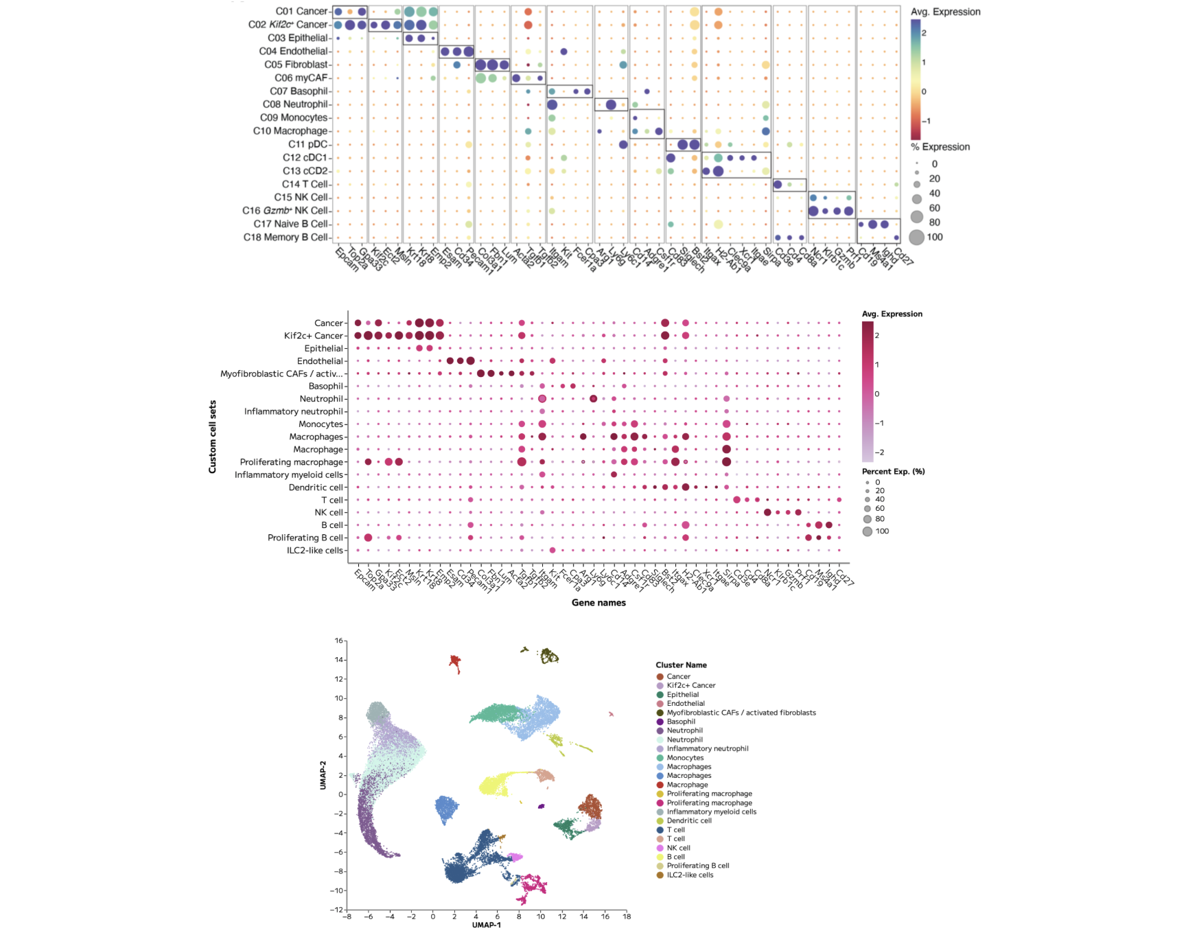
Figure 9: (Top) Cell type annotations and associated marker genes presented in the published paper. (Middle) A Trailmaker dot plot showing the same genes across our cell type annotations. (Bottom) The final UMAP showing annotated cell types.
Note that although there are some differences in the exact annotations that have been recreated, the core cell types are preserved.
Now that the cell types have been annotated, we can explore the biological differences between the experimental groups present within this dataset.
7. Explore differences between experimental groups
To start exploring differences between experimental groups, it’s common to use cell type abundance analysis and per cell type pseudobulk differential expression analysis, followed by pathway interpretation.
In Trailmaker’s Plots and Tables module, cell type abundance analysis can be performed using the Frequency plot.
In the tutorial dataset, we can easily plot cell type proportions across different metadata groups. Doing so gives critical insight into the dominant sources of variation between samples.
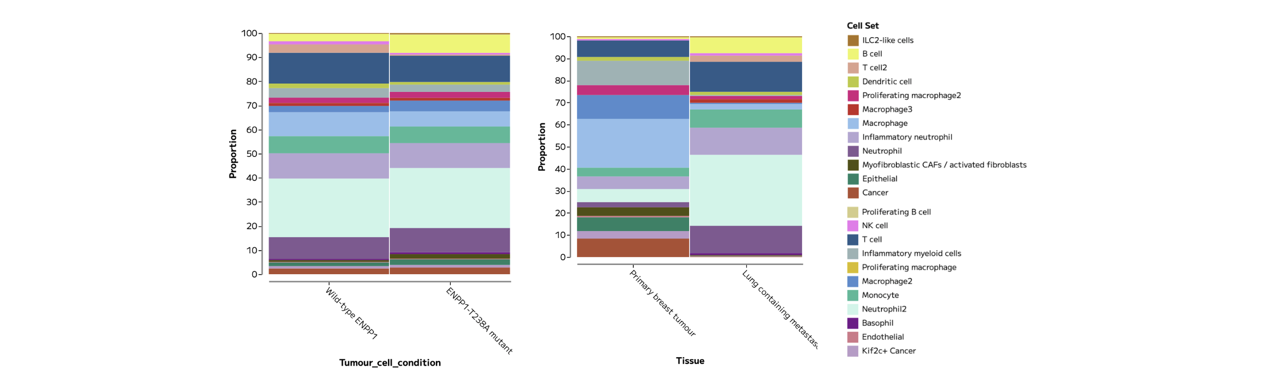
Figure 10: Frequency plots showing samples grouped by Tumour cell condition (left) and Tissue (right) show more pronounced differences in recovered cell type composition between tissues than between Tumour cell conditions.
When it comes to Differential Expression (DE) analysis, pseudobulk is widely considered the gold standard for single cell RNA-seq DE analysis because it compares biological replicates rather than treating cells as independent samples, reducing false positives while using well-established statistical methods relevant to sequencing data. Multiple cells within a sample are not a replacement for biological replicates.
Differential expression can be performed in Trailmaker’s Data Exploration module using the tab in the Lists tile.
Selecting to ‘Compare a selected cell set between samples/groups’ allows pseudobulk DE analysis between metadata groups. Following the findings in Figure 10, that Tissue is a large driver of variation in this dataset, we can calculate and visualise the top DE genes in the Primary breast tumours compared to the Lung containing metastases.
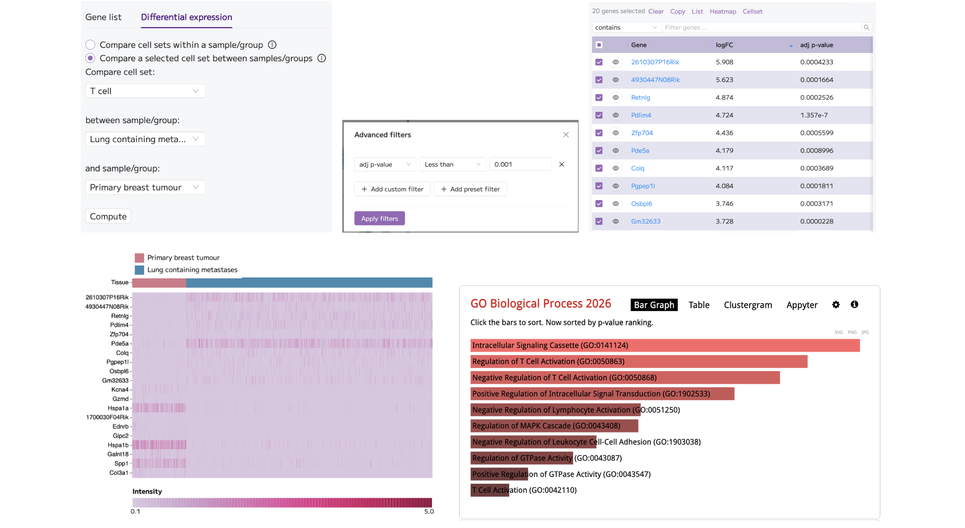
Figure 11: Performing differential expression analysis comparing Lung containing metastases to Primary breast tumours in T cells (top; left) and applying advanced filtering for the most significant genes, p<0.001 (top; middle) gives a list of gene results (top; right). The top 10 and bottom 10 genes, based on logFC, were selected and plotted on a Heatmap in the Plots and Tables module. The Heatmap was customised to show only T cells (bottom; left). The full list of filtered DE genes was sent for Pathway analysis using Enrichr, returning the GO Biological Process enrichment results that appear relevant to T cell function (bottom; right).
These provisional results provide a solid foundation for deeper exploration of the cell types, samples and metadata groups present in this dataset.
8. Create and export figures
The figures presented in this tutorial article (QC plots, UMAPs, Frequency plots, Dot plots, Violin plots and Heatmaps) were generated and customised in Trailmaker’s Plots and Tables module.
For this tutorial, re-create the following plots:
A UMAP coloured by annotated cell population.
A marker-expression dot plot or heatmap.
A Frequency plot comparing the composition of Custom cell sets across metadata groups.
A Heatmap of differentially expressed genes.
Customise the data presented on the plot using the ‘Select data’ menu. Alter the plot dimensions in ‘Main schema’ to ensure the labels are readable. Consider altering the colour choices or scales to best fit the needs of your plot presentation.
All plots can be exported as PNG or SVG image files using the 3 dot menu (...) at the top of the plot.
For advanced downstream analysis not supported within Trailmaker, download the AnnData (or Seurat, in other cases) object from the Insights project details page.
Common questions
Do I need to be a Parse customer?
Academic researchers can use Trailmaker free without being Parse customers. Trailmaker is also free for all Parse customers. You will need to create an account to access Trailmaker.
Can I upload 10x FASTQs?
No. For 10x Chromium data, upload supported processed gene-expression files to Insights. Generate those counts using an appropriate upstream workflow, such as Cell Ranger, before uploading supported files to Trailmaker’s Insights module.
What if uploading my own data fails?
Check that each sample contains the appropriate count matrix files, that they meet the supported format requirements, and that files from different samples have not been mixed or multiplexed. Follow the Trailmaker user guide for detailed requirements and troubleshooting.
Can I try Trailmaker without downloading these files?
Yes. You can explore public datasets in the Trailmaker data repository.
Summary
That’s it - you’ve gone from count matrices to figures in this guided tutorial for 10x Chromium data analysis.
Now you’re ready to start your own data analysis project!
Start exploring your own 10x Chromium data
You now have a route from processed count matrices to quality control, cell population exploration and figures—all without writing code.
Start your analysis in Trailmaker or explore the Getting Started guide for more help.
To build your understanding of the analysis steps, follow the free single-cell RNA-seq data analysis course.
Dataset credit: Wang et al., PNAS (2023), doi:10.1073/pnas.2313693120. Data available through GEO accession GSE233659.