

Cellenics® User Guide
We have prepared a user guide that will help you get the most out of the open source scRNA-seq data analysis and visualization tool, Cellenics®, using the Biomage-hosted community instance of Cellenics®.
As Cellenics® continues to be updated with new features and functionality, we will revise this guide on a regular basis. Be sure to check back for updates!
The table of contents provides quick access to each section of this user guide. To read a specific section, click on the appropriate heading of the section.
Getting Started with Cellenics®
Introduction to Cellenics®
Getting started with single cell RNA-sequencing (scRNA-seq) analysis can be daunting. You need familiarity with programming languages and sufficient bioinformatics knowledge (which can take months to study!) or time with a bioinformatician. But this process can be much faster and easier with Cellenics® an open-source, cloud-based analytics tool for scRNA-seq data!
Cellenics® allows you to explore and analyze your dataset without having to be proficient in programming. You can gain unprecedented insight into the cellular heterogeneity of complex biological systems and drive forward your research programme.
Biomage host a community instance of Cellenics®. Researchers studying cancer, cardiovascular health, and developmental biology use Cellenics® analysis software to make discoveries about complex biological systems. Your field could be next!
This guide will provide you with an introduction to Cellenics® and an overview of the features available in this open source tool.
Watch a 4-minute introductory demo of Cellenics® below!
Creating an account and logging in
Access the Biomage-hosted community instance of Cellenics® at: https://scp.biomage.net.
If you do not have an account yet, click “Sign Up” to create one. Creating an account takes only a few minutes. Provide your email address and name and set a password. You’ll need to verify your email address by clicking the link in the email we send to you when you sign up.
If you already have an account, simply input your email address and password to log in.

When you’ve logged in, you’ll be directed to the Data Management module of Cellenics®.
Navigation
When you’re logged into Cellenics®, you can navigate between the modules using the navigation bar on the left side:

Note that navigation to some modules may be restricted. For example, navigation to the downstream modules (Data Processing, Data Exploration and Plots & Tables) is dependent on the successful upload of data from one or more samples to the Data Management module.
Account settings
The account settings menu can be found in the top right corner:

In the account settings menu, you can change your name and password:

If you need to change the email address associated with your Cellenics® account, please post a message on the forum for Cellenics users https://community.biomage.net/ for assistance.
Sequencing output data types
Sequencing output files are usually in the form of FASTQ files or raw binary base call (BCL). BCL files require conversion to FASTQ format for most downstream analysis protocols. FASTQ files are large data files containing raw sequence data and quality scores. Neither BCL nor FASTQ files are directly compatible with Cellenics®.
Further processing of these files is required before the data can be explored in Cellenics®. Various software packages exist to help with the pre-processing. These packages first remove incomplete transcripts and duplicates. The cleaned reads are then aligned (matched) to a reference genome. Sequence alignment enables the identification and annotation of genes. The occurrence of these sequences is then counted, quantifying the transcript amount of a specific gene in a sample.
The choice of scRNA-seq technology dictates the software package(s) that can be used to process the FASTQ files. This is because different single-cell platforms construct different fragments, which require different methods to analyze.
Data generated using 10x Genomics Chromium technology is typically processed using Cell Ranger or 10x Cloud. Cell Ranger or 10x Cloud outputs 3 data files per sample:
barcodes.tsv - list of barcodes (UMIs) that are available in the sample
features.tsv or genes.tsv - list of features/genes that are recognized
matrix.mtx - a file representing a matrix containing the number of detected transcripts, with genes along the row and barcodes/cells along the column. This is called a count matrix.
These files represent the raw gene expression data from the sample.

Example of a count matrix (matrix.mtx file)
These files are directly compatible with Cellenics®. They can be directly uploaded to the Biomage-hosted community instance of Cellenics® (https://scp.biomage.net/) to further process, analyze, visualize and make sense of this data.
You can see a simple representation of the single-cell sequencing data analysis pipeline starting with the BCL files below.

Cellenics® also supports data generated with BD Rhapsody™ technology! The BD Rhapsody™ targeted assays create sequencing libraries from single-cell transcriptomes. The BD Rhapsody™ Analysis pipeline takes the FASTQ read files and reference files for gene alignment. The pipeline filters by read quality, annotates R1 and R2 reads, annotates molecules, determines putative cells, selects the sample of origin (sample multiplexing only), and generates expression matrices. These expression sparse matrices as expression_data.st or expression_data.st.gz can be directly uploaded to the Biomage-hosted community instance of Cellenics® (https://scp.biomage.net/).
Data Management
Overview
The next step after creating your account with the Biomage-hosted community instance of Cellenics® (https://scp.biomage.net/) is to start a new project and upload your data. This is a detailed step-by-step guide to the Data Management module where these actions are performed.
The Data Management module is where you can view and edit existing projects and the sample data and metadata within each project, and upload new data and metadata to existing or new projects.
You can watch a short video below that provides an overview of the Data Management module!
Navigation
After logging into the Biomage-hosted community instance of Cellenics® (https://scp.biomage.net/), you will be directed to the Data Management page.
A list of all available projects in your account is displayed in the Data Management module, along with details about the selected project. Among these details are project name, description, sample list, and associated data and metadata:

New users will see an empty project list and can either opt to explore our repository of example datasets or create a new project to get started:

Data format conversion for Cellenics®
To upload your data to the Biomage-hosted community instance of Cellenics® (https://scp.biomage.net/), you'll need the raw count matrices in the shape of three files: barcodes.tsv, features.tsv and matrix.mtx files. In case your data is in another format, our team has prepared tutorials on how to convert various other data formats.
If you are dealing with an object that hasn't been listed below and you're not sure how to convert it, please post a message on the forum for Cellenics users https://community.biomage.net/ for assistance.
Count matrix stored in .rds file
Tutorial on how to demultiplex a count matrix stored in an R data files (.rds) object and convert it to features/genes.tsv, barcodes.tsv and matrix.mtx.
https://www.biomage.net/blog/how-to-demultiplex-an-rds-object-and-convert-it-to-10x-files
HDF5 file
Tutorial on how to convert H5 files to features/genes.tsv, barcodes.tsv and matrix.mtx.
https://www.biomage.net/blog/converting-h5-files-to-upload-to-cellenics
Seurat object stored in .rds file:
Tutorial on how to demultiplex a Seurat object stored in an R data files (.rds) object and convert it to features/genes.tsv, barcodes.tsv and matrix.mtx.
https://www.biomage.net/blog/how-to-demultiplex-a-seurat-object-and-convert-it-to-10x-files
Tabular data in a CSV/TSV file
Tutorial on how to convert CSV/TSV files to features/genes.tsv, barcodes.tsv and matrix.mtx.
https://www.biomage.net/blog/converting-csv-to-upload-to-cellenics
Exploring an example dataset
Cellenics® provides a repository of several example datasets that you can use to get started. To access the public dataset repository click on the “Get started using one of our example datasets!” button in the Project Details view.

Alternatively, click on the “Create New Project” button, and then choose ‘Select from Dataset Repository’.

You are going to be redirected to our public dataset repository. To use a dataset, click on the “Explore” button.

The dataset is going to be automatically added to your Project list.

Creating a new project to upload your own data
If you have your own dataset that you’d like to upload and explore, click on the “Create New Project” button to create a project. Then select the option ‘Upload project’.


Now, you can name your project and add a project description (optional). Note that the project name must be different from other projects in your account.

Changing project name
Projects can be easily renamed in the list of projects by clicking on the editing button next to the project name.

Input the new project name and click save.

Uploading 10x Chromium data
Once you have created a project, you can upload your own data.
Samples that you want to analyze together should be uploaded to a single project. Add samples to the new project by clicking on the “Add Samples” button.

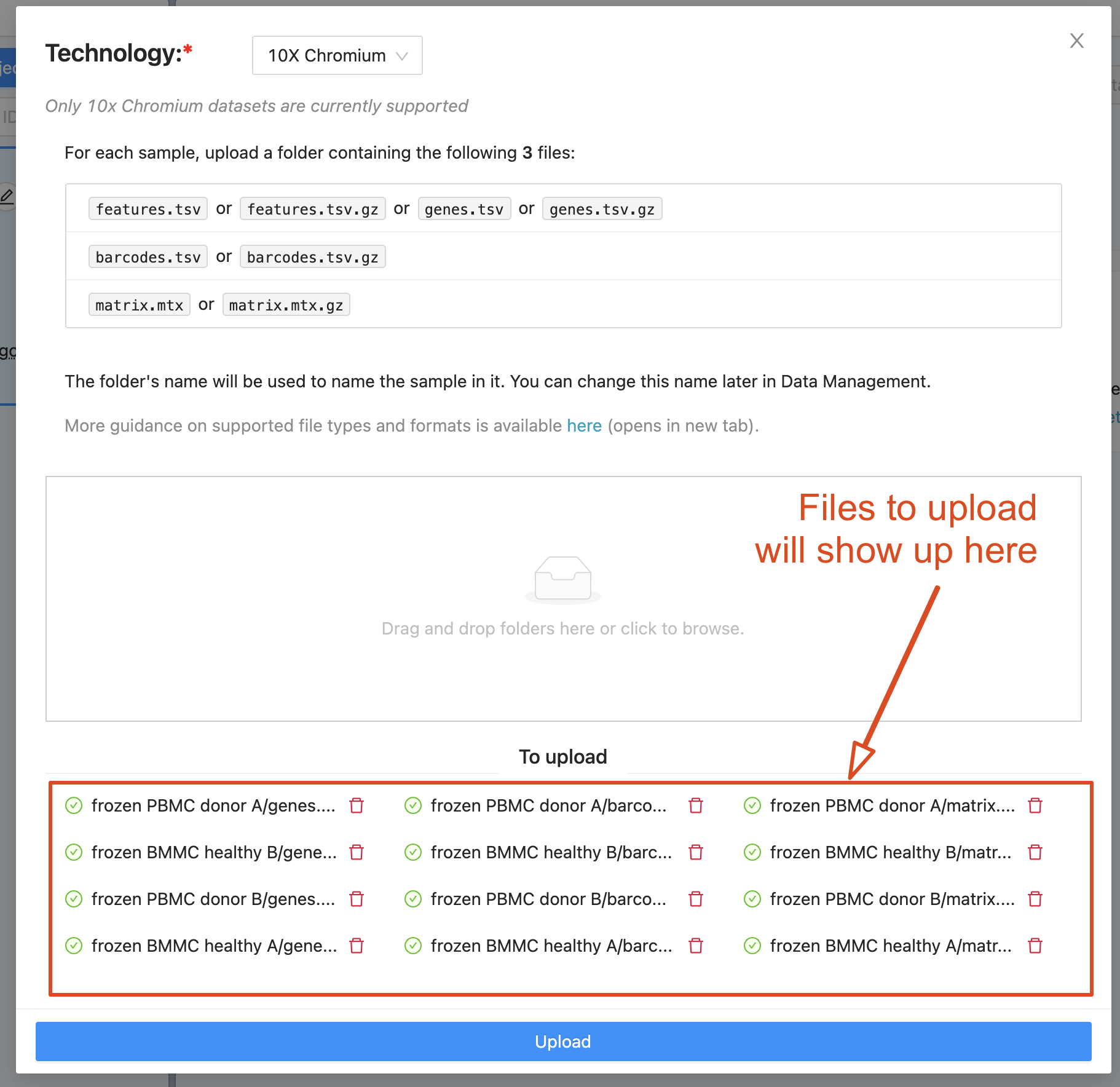
The file upload modal will then appear. To add the samples, drag and drop the sample folders. Within each sample folder, you should provide 3 files - features/genes, barcodes and matrix. The files are usually in gunzipped format i.e. ending in .gz. Normally, these 3 files associated with a given sample are in a folder that is named with the sample ID. Cellenics® will use each folder’s name as the sample name. The sample names are not fixed and can be easily changed in the list of samples after upload.
You can find more information about format conversions here.

Files selected for upload will show up in the modal. You can remove unwanted files using the delete icon that appears next to each file. Click “Upload” to start the upload process. Note that multiple samples can be uploaded at the same time.
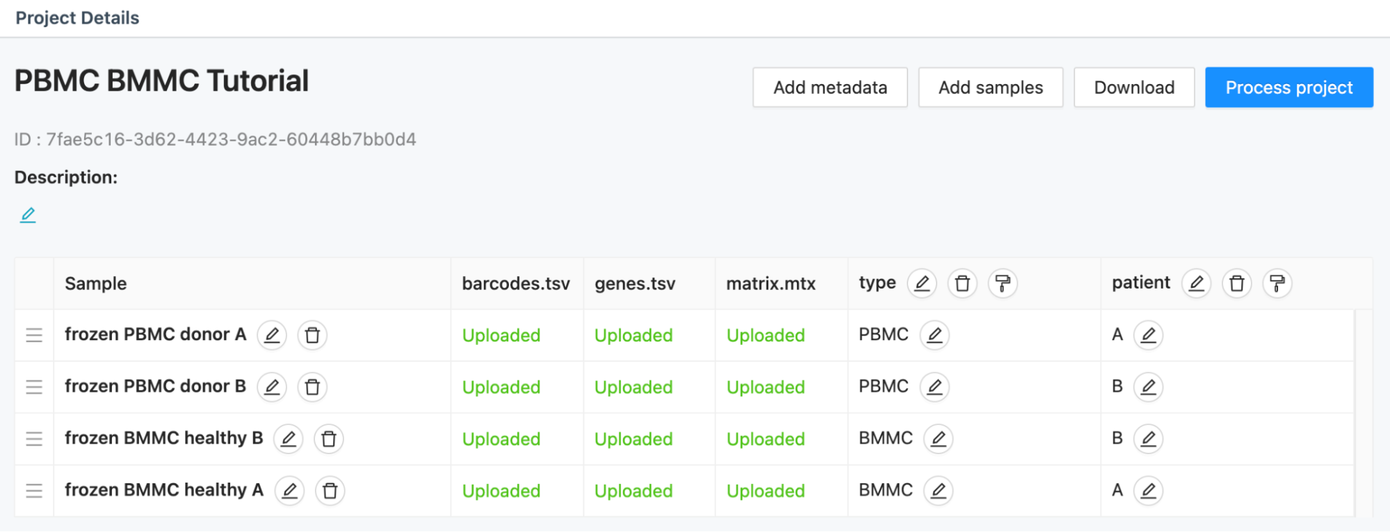
The files will be compressed (if not yet so) before uploading. You can see the status of the upload for each file from the upload bar. Files that are getting compressed appear in orange. Successfully uploaded files appear in green. Files that fail to upload will show in red. Examples of these file upload statuses are shown below:


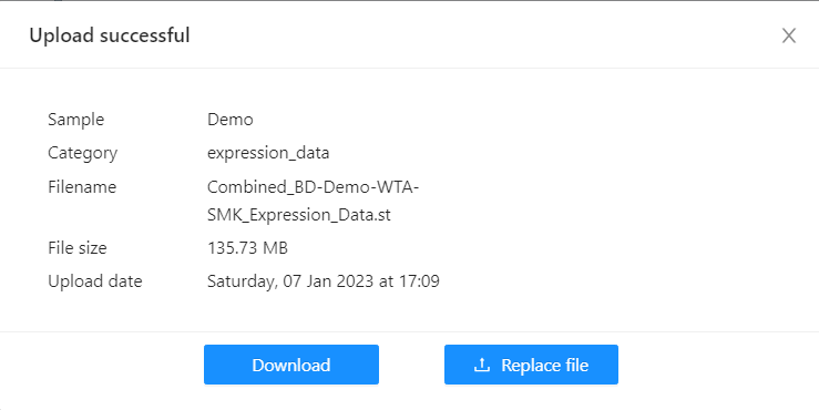
You can click on the “Uploaded” or “Upload error” text of the specific sample to see the details of the file. In the case of a successful upload, you will be able to download or replace the file. In case of a failed upload, the modal will show options to retry the upload or replace the file. Both examples are shown below:

Once sample files have been uploaded, you can re-order samples in the sample list. Drag the sample to the desired position by using the button (3 lines) on the left of the sample name. The sample order in the Data Management module determines the order that samples appear in the other modules of Cellenics®. Sample order can be changed later in the Data Exploration module.
Adding metadata
The addition of metadata is important for multi-sample experiments in order to assign samples to groups. For example, samples within a dataset could be assigned as “control” and “treated”; or “healthy” and “disease”. Assigning metadata will then allow the comparison of groups to determine differentially expressed genes (e.g. to calculate differentially expressed in genes in a cluster of interest comparing two groups) and visualization of groups (e.g. a dot plot showing the expression of multiple genes of interest across two or more groups) further downstream in the platform.
Once the samples are uploaded, you can add metadata to the samples by clicking the “Add Metadata” button and “Create track”. You will be asked to name the “metadata track”. This results in a column being added to the sample information table. Metadata can be assigned to each sample.
For example, you might label the metadata track “Treatment” and assign each sample as “control” or “treated”. Alternatively, you might label the metadata track “Tissue” and assign each sample as “blood” or “skin”. There is no limit to the number of metadata tracks that you can add to a project.

Once all the metadata has been inserted, click on “Process project” and confirm by clicking “Yes”. This will launch your data analysis.

Alternatively, you can upload a tab-separated file (.tsv) with all the metadata information you need to add, and Cellenics® will take care of the rest. To do so, click the “Add Metadata” button and “Upload file”.

In the pop-up, add your metadata files and click Upload.

Uploading BD Rhapsody data
Cellenics® now supports data generated with BD Rhapsody™ technology! Once you have created a project, you can upload your own data.
Samples that you want to analyze together should be uploaded to a single project. Add samples to the new project by clicking on the “Add Samples” button.

The file upload modal will then appear. Change the technology used from 10x Chromium to BD Rhapsody in the drop-down menu.
To add the samples, drag and drop the sample folders. Within each sample folder, you should have expression_data.st or expression_data.st.gz data. Cellenics® will use each folder’s name as the sample name. The sample names are not fixed and can be easily changed in the list of samples after upload.
The zip files that are output by the primary processing pipeline contain the .st files that should be uploaded and they must be unzipped first. The folder with Multiplet and Undetermined cells should not be uploaded since it would distort the analysis.

Files selected for upload will show up in the modal. You can remove unwanted files using the delete icon that appears next to each file. Click “Upload” to start the upload process. Note that multiple samples can be uploaded at the same time.

If you have AbSeq data, it is filtered out by default. After clicking upload, you can check the box to include the AbSeq data. Support for AbSeq is currently for visualization purposes only, as experiment-wide normalization will be slightly skewed. In case there is AbSeq data in your experiment, we suggest you create two projects; one including AbSeq data and one without, and compare the results.

The files will be compressed (if not yet so) before uploading. You can see the status of the upload for each file from the upload bar. Files that are getting compressed appear in orange. Successfully uploaded files appear in green. Files that fail to upload will show in red. Examples of these file upload statuses are shown below:


You can click on the “Uploaded” or “Upload error” text of the specific sample to see the details of the file. In the case of a successful upload, you will be able to download or replace the file. In case of a failed upload, the modal will show options to retry the upload or replace the file. An example of successful upload is show below:
Once sample files have been uploaded, you can re-order samples in the sample list. Drag the sample to the desired position by using the button (3 lines) on the left of the sample name. The sample order in the Data Management module determines the order that samples appear in the other modules of Cellenics®. Sample order can be changed later in the Data Exploration module.
Launching an analysis
Clicking on the “Process project” button initiates the conversion of the count matrices into a Seurat object Sample names and metadata that were input in the Data Management module are inserted into the Seurat object.
The progress of this conversion process is displayed to the user on the interface. This step might take some time for large datasets, so you can opt to get notified via email once this step is completed and leave the screen.

The generation of the Seurat object is an essential prerequisite to all downstream analysis in Cellenics®. If the generation of the Seurat object fails, you will see an error screen like the one below. You can try to re-run the process or return to Data Management where you can choose to launch another analysis.

If the generation of the Seurat object completes successfully, the Data Processing pipeline will be triggered automatically to run using our automatically determined settings. For more information, see the chapter of this user guide that’s dedicated to the Data Processing module.
Share a project
Projects can be shared with colleagues or collaborators using the “Share” button in the Data Management module.
You will remain the owner of the project: owners have control over the upload of sample data, the addition of metadata, the running of the Data Processing pipeline, and the sharing of projects.
Anyone you share a project with will have explorer roles: explorers can use the Data Exploration and Plots and Tables modules, but cannot make any changes to samples or metadata in the Data Management module or re-run the pipeline in the Data Processing module.

In the sharing pop-up, you can input the email addresses of your collaborators. Additionally, you can revoke access to the project for specific collaborators in the same modal.

Copy a project
The 'Copy' button in the Data Management module allows you to quickly and easily create a copy of an existing project. In doing so, you can create multiple versions of analysis of a dataset, for example, to compare different data processing settings side-by-side.
Click ‘Copy’ and a copy of your project is going to appear automatically. The copy of the project is named automatically as well. You can rename the copy of the project as shown in the Changing project name section.
You will have to process your project copy as a new project.


Downloading data from a project
The features, barcodes and matrix files for each sample can be downloaded from the sample list view by clicking on the green ‘Uploaded’ text for each file.
Raw and processed Seurat objects can be downloaded as R data files (.rds) using the ‘Download’ button at the top of the Project Details panel of the Data Management module.

Deleting a project
If you wish to delete a project, click on the delete button next to the project name.

Since deleting a project cannot be undone, a pop-up will appear asking for confirmation. If you are still sure you want to delete a project, type in the name of the project at the bottom of the pop-up to confirm the deletion and click ‘Permanently delete project’. If you don’t want to delete the project, just click ‘Keep project’.

Data Processing
Overview
Data generated from a single cell RNA-sequencing experiment always requires processing to clean the data. During data processing, empty droplets, dead cells, doublets and poor quality cells are excluded from the downstream analysis. These steps ensure that the processed data are high quality and return accurate results during downstream analysis.
After data upload, you will be prompted to process your project. Cellenics® applies a default data processing pipeline to your dataset in the Data Processing module to prepare it for downstream analysis and visualization. The default pipeline applies sensible default settings to your dataset so that you can immediately access and explore the first pass of the analysis. All data processing settings can be adjusted to your preferences.
The Cellenics® data processing pipeline consists of 7 linear steps. The output of each step in this module becomes the input for the next step. Steps 1-5 consist of filters to remove unwanted and poor quality data from each individual sample. In step 6, multiple sample datasets are integrated to remove batch effects, and dimensionality reduction is performed. Finally, in step 7, the embedding is configured (e.g. UMAP or t-SNE) and clustering is applied.
The filtered, integrated data with clustering is then available for downstream exploration and visualization in the Data Exploration and Plots and Tables modules.
You can watch a short video below that provides an overview of the Data Processing module!
Automated data processing pipeline
In the Data Management module of Cellenics®, the data processing pipeline is triggered by the ‘Process Project’ button. This first run of the data processing pipeline uses default settings to set sensible thresholds for filtering, and standard settings for integration and clustering.
The automated data processing pipeline values are established according either to the current best practice in the field or according to the spread of each sample data. Specific details on the default values for each step in the data processing pipeline can be found in the Data Processing Steps section.
Pipeline status indicator
At the top right of the page in the Data Processing module, there is a pipeline status indicator. When the data processing pipeline is complete, the pipeline status indicator will appear green (screenshot A, below), whilst steps that are in progress appear gray (screenshot B). If the pipeline fails, the indicator will appear incomplete and marked as failed (screenshot C). The step that is currently being viewed is marked in orange (screenshots A-C).


For more information on what to do if your pipeline fails, see the Pipeline Failures section.
Navigating through the data processing steps
Cellenics® has the following steps in the Data Processing module:
1. Classifier filter
2. Cell size distribution filter
3. Mitochondrial content filter
4. Number of Genes vs UMIs filter
5. Doublet filter
6. Data integration
7. Configure embedding
You can navigate between these filters using the dropdown menu on the top left of the page or the navigation arrows on the top right of the page.
The dropdown menu and the status bar also show if the step is completed or not. Steps with a check mark (✔) to the left are complete; steps with a cross mark (❌) to the left have failed.
Filtering steps (1-5) can be disabled using the ‘Disable’ button at the top of the page. Filtering steps that are disabled are shown in the dropdown menu with the step name in strikethrough.

In filtering steps 1-5, the samples available within the project are shown one after another with one plot for each sample. You can scroll through the samples easily. Individual sample plots can be minimized by clicking on the sample name above the plot.
Data processing plots and statistics
For the filtering steps (steps 1-5), data is filtered on a per sample basis. A plot is shown for each individual sample within each filter. Each plot can be fully customized to your design preferences using the ‘Plot styling’ menu. Below each sample plot, there is a table that describes the filtering statistics for each sample: ‘# before’ describes the number of cells present in the sample before the current filtering step; ‘# after’ describes the number of cells present in the sample after the current filtering step; ‘% changed’ describes the proportion change in cell number as a result of the current filtering step.
An example filtering plot and associated statistics table for a single sample in filtering step 4 is shown below as an example:

Data Processing steps
Step 1: Classifier filter
The classifier filter aims to exclude empty droplets and retain droplets that contain cells. To achieve this, the filter uses the ‘emptydrops’ method to calculate the False Discovery Rate (FDR), a statistical value which represents the probability that a droplet is empty (read more about this method here). The default FDR value is 0.01 for all samples. Only droplets with FDR < 0.01 are retained. Therefore, in this step, droplets with low FDR are retained for downstream analysis, whilst droplets with a high FDR are removed from downstream analysis.
Two plots are provided to visualize the data. The first plot is a knee plot that determines the FDR threshold for considering cells valid for analysis. The knee plot ranks cells by the number of distinct unique molecular identifiers (UMIs) for each barcode on a logarithmic scale. Using the log value of the UMIs exposes a “knee” on the graph curve where the number of UMIs decreases. The turning point in the “knee” is usually used as the point to set the FDR threshold. Cells with low UMI counts contain fewer transcripts, and there is a higher probability that the cells are empty drops. Therefore we would like to filter cells that are above the FDR threshold (orange) out. The cells in the green region have an FDR<0.01 and are retained. The gray “mixed” region contains some cells that are retained and some cells that are filtered out.

The second plot is an “empty drops plot”. This is an alternative visualization of the data which plots the number of UMIs against the probability that the cell is an empty drop. The red line shows the threshold value that is set to filter the cells. Cells below this red line are retained, while cells above the red line are excluded from downstream analysis.

Note that for datasets that have been pre-filtered (e.g. in Cell Ranger) the Classifier filter is disabled and there are no plots to view.
The default FDR value is set to 0.01 in this filtering step. This is the standard threshold used for the emptydrops method. Although it is possible to override this setting, we do not recommend that you do so.
Step 2: Cell size distribution filter
The cell size distribution filter can be used to fine-tune the classifier filter, by further discarding droplets that are likely to be empty. Unlike the classifier filter which works on probability, this filter sets a hard threshold on the minimum number of UMIs contained in a droplet in order for that droplet to be considered a real cell. Hence, cells with UMIs lower than this threshold are filtered out.
In Cellenics®, this filter is disabled by default because most of the time, the output of the classifier filter is good enough not to warrant further refinement. This means you will see a blue information box above the samples reminding you that this filter is disabled, as well as a strikethrough of the filter name in the dropdown menu. Although this filter is disabled by default, the plots are still generated to visualize the state of the data and you can decide to switch this filter on using the ‘Enable’ button at the top of the page.
The data for this filter is visualized as a knee plot. The plot ranks cells according to the number of UMIs on a logarithmic scale. The inflection point around the “knee” signifies the threshold at which the number of UMIs in a cell changes drastically. Note that the cell rank on the x-axis is on a logarithmic scale, which means the area under the curve does not proportionally represent the number of cells that are filtered / unfiltered.

The second plot view in this filter is a histogram that shows the number of cells that are affected by the cell size distribution filter. This histogram visualizes cells below (orange) and above (green) the set threshold. The orange cells are filtered out of the dataset whereas the green cells are retained. If the histogram plot shows a binomial distribution then consider switching on this filter. For example, in the histogram plot below the cells identified in orange may in fact be empty droplets and you should consider filtering them out.

You may decide to switch on this filter in order to set a minimum number of UMIs threshold for your dataset. To do so, click on the ‘Enable’ button at the top of the page, then set the desired value(s) for each sample. You will then need to re-run the pipeline in order to apply the changes.
Step 3: Mitochondrial content filter
Droplets may contain live or dead cells. The mitochondria of dead cells rupture, spilling out transcripts of mitochondrial genes into the cell. The presence of these mitochondrial gene sequences can skew the analysis results, as transcripts from live cells are often of interest rather than transcripts of dead cells. Thus, for most datasets it is advisable to filter out dead cells from the analysis.
The mitochondrial content filter removes droplets containing dead and low-quality cells by looking at the percentage of mitochondrial transcripts contained in the droplet and setting an appropriate threshold. Droplets with mitochondrial content higher than the threshold are removed from downstream analysis.
The default threshold for the proportion of mitochondrial genes is calculated per sample. The typical cut-off range is 10-50% of mitochondrial reads per cell, with the default cut-off in Cellenics® determined as 3 median absolute deviations above the median.
Two plot views are available in this filter. The first plot is a histogram which shows percentages of mitochondrial reads and their corresponding proportions of cells. The percentage of mitochondrial reads is the percentage of UMIs mapped to mitochondrial genes from total UMIs. Dead cells (blue) are filtered out and live cells (green) are retained.

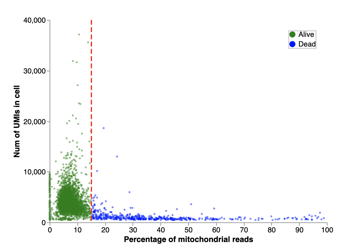
The second plot is a scatter plot which shows the total number of UMIs in each cell plotted against the percentage of mitochondrial reads. Each dot in this plot is an individual cell. As in the previous plot, the dead cells are filtered out (blue) and live cells (green) are retained.
Step 4: Number of genes vs UMIs filter
The number of genes vs UMIs filter works on the principle that the number of unique transcripts (as marked by the number of UMIs) increases linearly with the number of genes. Droplets that deviate from this linear relationship fall into one of two categories:
(1) Droplets contain a lot of genes but few UMIs. This means transcripts in the droplet are not amplified well.
(2) Droplets contain few genes but a lot of UMIs. This means that the few transcripts that exist are over-amplified.
This filter visualizes the data using a scatter plot to map the number of gene counts on a logarithmic scale against the number of UMIs (molecules) on a logarithmic scale. The range of acceptable data points is defined with 2 linear thresholds, signified by red lines. Cells not located between the two red lines are considered outliers and are filtered out.
The scatter plot is interactive - moving the red prediction interval lines will help you to choose the most appropriate value to filter cells in your samples. To do so override the automatic settings as shown in Adjusting a data processing setting section, and use the prediction interval slider to choose your preferred values.

If one or more samples in your dataset contains a separate population of cells in this filter plot, such as in the example plot above, then we recommend further investigating the population to determine if it should be excluded or retained. One way to do this is to disable the filter (using the ‘Disable’ button at the top of the page) which will retain all cells for downstream analysis, and allow you to further investigate the secondary population in downstream modules in Cellenics®.
Step 5: Doublet filter
Doublets contain the content of multiple cells in a single droplet, leading to skewed data and false conclusions, especially concerning cellular heterogeneity and identity. Doublets usually arise due to errors in cell sorting or capture.
The doublet filter calculates the probability of a droplet being a doublet and filters out cells with a high probability of being a doublet. Calculation of the probability is carried out using the scDblFinder algorithm (a detailed explanation of this method can be found here).
This filter sets a hard threshold above which droplets are filtered out. This threshold is marked by the red line in the provided plot for this filter. The plot shows the proportions of cells and their corresponding probabilities of being doublets.

For samples that contain few cells, the calculation of doublet score probabilities has less power and, therefore, tends to show more cells with an intermediate score between 0.2 and 0.8.
Step 6: Data integration
The Data Integration step removes batch effects and reduces the dimensionality of the data.
Batch effects are variations caused by differences in experimental conditions, introducing noise which skews the true variation for a sample. Runs of different samples have different values of noise. Hence, comparing these samples directly without addressing batch effects would compound the noise. Removing batch effects enables comparison and composition of samples analyzed in different runs with minimized error. In essence, batch effect correction ensures that downstream analysis focuses on real biological differences between samples, rather than irrelevant sample-to-sample or batch-to-batch variation.
Three data integration methods are available – Harmony, Fast MNN, and Seurat v4. Harmony is selected as default. However, you can select the integration method and set the controls based on your requirements. Normalization is applied to each sample before integration. There are several methods to achieve normalization; the default method in Cellenics® is LogNormalize. "SCTransform" claims to recover sharper biological distinction compared to log-normalization. SCTransform can only be applied when the integration method is set to Seurat v4.
Dimensionality reduction reduces the complexity of the dataset while preserving variation. In essence, dimensionality reduction “compresses” the data to enable visualization in 2 dimensions. There are many methods of dimensionality reduction, but one of the most popular in the field is Principal Component Analysis (PCA). This method introduces principal components (PCs) - a linear combination of variables in the data that better explain variations. The largest variance is accounted for by the first PC, the second largest variance by the second PC, and so on.
PCA is great for high dimensional data, but it is not optimized to generate 2-dimensional embedding. In practice, PCA is used to reduce the raw data into a lower dimension, acting as a pre-processing step. The resulting data is fed into other dimensional reduction algorithms, such as UMAP or t-SNE, to reduce the data into 2 dimensions.
Normalization can be biased by certain gene categories, such as ribosomal, mitochondrial and cell cycle genes. In data integration, these three gene categories can be excluded from the analysis. For example, cell cycle genes should be removed if sampling timepoints occurred throughout the day. Those genes can otherwise introduce within-cell-type heterogeneity that can obscure the differences in expression between cell types. To mitigate this, cell cycle genes can be excluded from the analysis of human and mouse species under ‘Dimensionality reduction settings’.
There are 3 plot views available in the data integration step. To change the plot type, select the desired plot under the plot view section.

The first plot is a preview of the embedding generated after the dimensional reduction. This plot is only available for multi-sample datasets, and is not available in projects with only one sample.

The second plot is a frequency plot which shows the contribution of each sample to each cluster. This plot is also only available in projects with multiple samples.
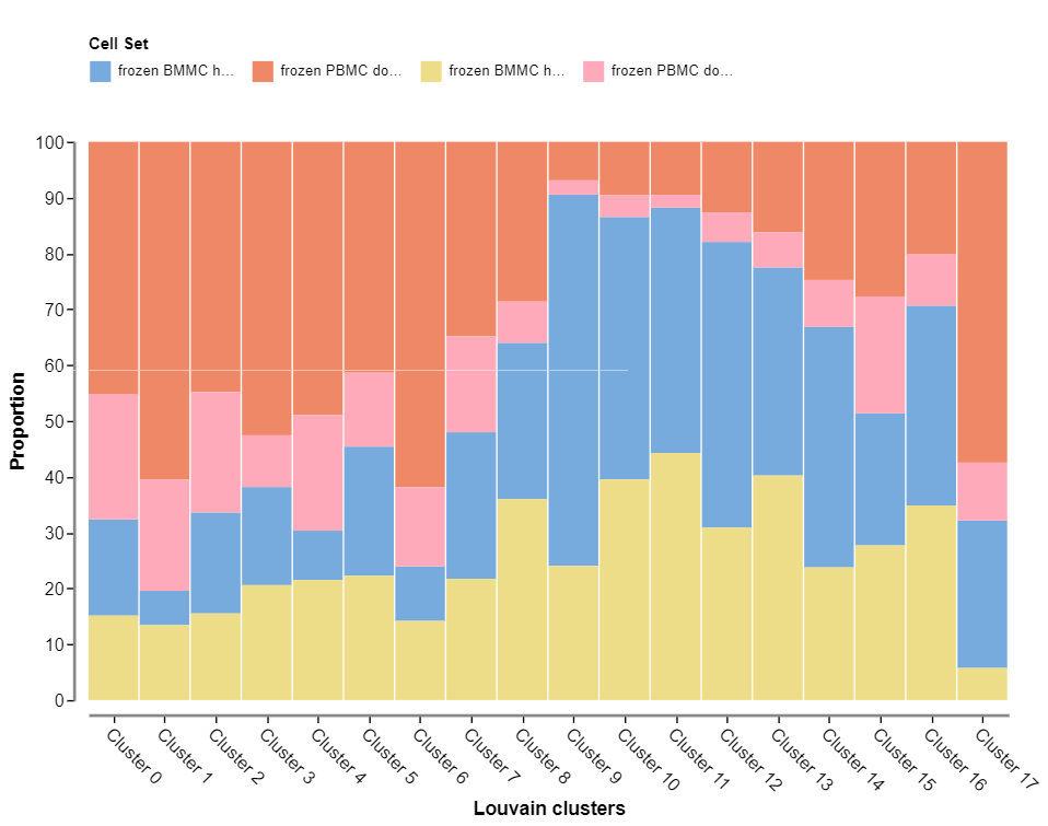
These first two plot views allow you to assess the quality of the integration of multi-sample datasets. Well integrated datasets will display good distribution of each sample across all clusters.
The third plot is an elbow plot which maps the percentage contribution of each Principle Component (PC) to the total variation in the dataset. The default setting for the number of PCs is defined by Cellenics® as the number of PCs that explains 85% of the variation (if less than 30 PCs), or 30 PCs.

Downsampling
Large datasets (e.g. >100,000 cells) can be downsampled specifically for the integration step. This speeds up the time it takes to integrate large datasets using some methods (especially Seurat_v4 and FastMNN) and enables large datasets to successfully complete the pipeline. Once the data are integrated, the full data are available for downstream analysis and visualization.
Geometric sketching finds random subsamples of a dataset that preserve the underlying geometry, which is described in this paper: Geometric sketching compactly summarizes the single-cell transcriptomic landscape. In short, geometric sketching divides the transcriptional space into variable-sized hypercubes and then randomly samples the same amount of cells from each of the cubes; the resulting sketches preserve the data structure and put more emphasis on small and underrepresented cell types, leading to improvements even over using the whole dataset.
You can downsample your data under Downsampling Options.

Then change the Method to Geometric sketching. If you wish, you can also change the percentage of cells to keep.


Step 7: Configure embedding
In the last step of the Data Processing module, integrated data is further reduced into a 2-dimensional embedding. An embedding is a space which allows for the translation of data of a high dimension into a low dimensional space. High dimensional data represents a data set where the number of features is higher than the number of samples. The low dimensional space should represent the meaningful properties of the high dimensional data.
Cellenics® provides two methods to visualize embedding: UMAP and tSNE. UMAP is a more recent technique with an algorithm that is more readily adjustable to parallelization and works faster than tSNE. Hence, UMAP scales better for large datasets compared to tSNE. Generally, it is recommended to use UMAP embedding to visualize your data.
After creating the embedding, the embedded data points are clustered and colored according to those cluster annotations. Clustering is the process of grouping cells of high similarity. There are several clustering methods available, but the most used are Louvain and Leiden methods. Cellenics® uses the Louvain clustering method by default. Clusters are color-coded and numbered numerically so they can be identified and explored in downstream analysis in Cellenics®.
The clustering result can be modified by adjusting the clustering resolution in the clustering settings menu in step 7 of the Data Processing module. The embedding and clustering results that are produced in this step propagate the Data Exploration and Plots & Tables modules of Cellenics®.
There are six plot views available in step 7 where the embedding and clustering settings are configured. To change the type of the embedding plot, select the desired plot under the plot view section.

The first plot shows a UMAP embedding by default, showing cells from all samples clustered and colored according to the Louvain clustering algorithm:

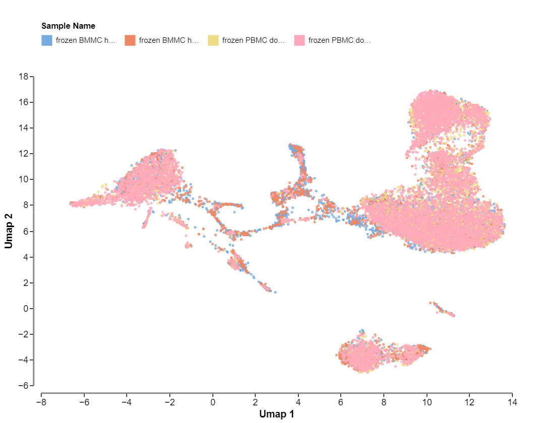
The second plot shows the same UMAP embedding, but coloured by sample. This plot shows the distribution of samples across clusters in the embedding. When there is only one sample in a dataset, this plot is unavailable. With a multi-sample dataset, this is what the plot will look like:
The rest of the plots show quality control data plotted on the UMAP embedding. The third plot shows the distribution of the mitochondrial genes. Ideally, this plot should show uniform color across all clusters and throughout the embedding, meaning that all the cells contain a similar average number of mitochondrial content. If high mitochondrial content is concentrated in one cluster, this would suggest that there is a population of dead cells that is clustered together. In this case, we recommend returning to the mitochondrial content filter (step 3) and reduce the threshold of the percentage of mitochondrial reads to try to remove the cluster.

The fourth plot shows a UMAP embedding coloured by the doublet probability score. Ideally, this plot should show a uniform distribution of color. Similar to the third plot, you should look for any specific cluster that has high coloring of doublet score, which would indicate a population of doublets still present in the data. In this case, we recommend returning to the doublet filter (step 5) and adjusting the doublet score threshold.

The fifth plot shows a UMAP embedding coloured by the number of genes.

The sixth plot shows a UMAP embedding coloured by the number of UMIs.

Adjusting a data processing setting
The default settings for each data processing step can be overridden using the ‘manual’ button in the Filtering Settings menu that is available within each step. For filtering steps 1-5, the setting can be altered for one specific sample or the adjusted setting can be applied to all samples using the ‘Copy to all samples’ button.

Specific filtering steps (steps 1-5) can be disabled using the ‘Disable’ button at the top of the filter. Using this button will switch off the selected filter so that no cells are filtered out at this step, and all cells are taken forward to the next step of data processing.

When a data processing setting is adjusted or a filter is disabled, you will be prompted to re-run the data processing pipeline. You can elect to ‘Run’ the pipeline or ‘Discard’ the changes. When the pipeline reruns, only the steps that have adjusted settings will be re-run. Note that re-running the data processing pipeline is likely to take several minutes, with the exact time dependent on the size of your dataset.

Pipeline failures
It’s important to note that the data processing steps may fail if there is not enough data to be processed. Steps 1-5 in the pipeline can fail if the number of cells is very low, and the data integration step (step 6) can fail if the number of cells is lower than 100.
If this happens and your pipeline fails, there are several ways that you can address this problem:
Reduce the number of cells being filtered out: You can alter the filtering settings in steps 1-5 (e.g. by lowering thresholds) or disable specific filters to reduce the number of cells that are filtered out which will, therefore, increase the number of cells proceeding to downstream processing and analysis. However, this can lead to poor quality cells being included in the downstream analysis.
Elect to use no integration: You can select ‘No integration’ in the data integration settings in step 6. This may result in a successful pipeline run, however, there may be significant batch effects that have not been removed from the analysis.
Exclude the sample(s) with too few cells: It is possible to exclude the problem sample(s) that has too few cells. This can be done in the existing project by setting a high threshold in one of the filtering steps in order to filter out 100% of the cells in that sample. Alternatively, you could delete the problem sample(s) in the Data Management module in the existing project or create a new project and upload only the other samples, excluding the sample(s) with few cells.
If your pipeline fails and you are not sure how to fix the issue, please post a message on the forum for Cellenics users https://community.biomage.net/ for assistance.
Saving a processed project
Whilst the project is being processed, you can leave the screen, log out of the Biomage-hosted community instance of Cellenics® and close your web browser without affecting the processing - the data processing pipeline will continue to run. You can elect to receive an email confirmation when your data processing pipeline completes using the ‘Receive email notifications’ toggle button when you first process a project.
The processed project is saved automatically by the Biomage-hosted community instance of Cellenics®. When you log out and then return to the platform, you can immediately view the processed project.
Exporting the data processing plots
All plots that are available in the data processing module can be fully customized using the ‘Plot styling’ menu. You may want to consider including these quality control plots in your manuscript as evidence of sample quality.
To download a plot from the data processing module, select the ‘...’ menu on the top right of the plot. Download options include SVG (high resolution) and PNG (lower resolution).

Downloading the data processing settings
All data processing settings can be downloaded as a text file (.txt) using the ‘Download’ button in the Data Management module.
We recommend that you report these data processing settings (filtering thresholds, integration method, etc.) in your manuscripts. We can assist with writing this paragraph, if needed - please post a message on the forum for Cellenics users https://community.biomage.net/ for assistance.
Summary
The Data Processing module in Cellenics® filters out empty droplets, dead cells, doublets and low-quality cells, removes batch effects and reduces the dimensionality of the data. This module is an essential prerequisite for downstream data analysis and visualization.
Now that your data is processed, it’s ready to be explored in the Data Exploration module!
Data Exploration
Overview
The Data Exploration module of Cellenics® has a wide variety of features for in-depth exploration of your data. Using this module, users can identify which cell types are represented by their cell sets, fully customize cell set selection, and generate insight into the dataset using gene expression visualization and differential expression.
Custom cell sets can be created using selection tools, based on the expression of one or more genes, or by manipulating the default Louvain clusters. It's easy to rename clusters or recolor by sample, metadata, or gene. Standard analysis actions such as marker heatmap and UMAP are pre-loaded. Cell set annotation can be done manually using the marker heatmap and differential expression features or automatically using the scType annotation method.
Users can calculate differential expression between cell sets within a sample/group or compare a cell set between samples and groups. Differential expression results can be filtered further, for example, by selecting only upregulated genes. Users can perform pathway analysis on the list of differentially expressed genes using external services - Pantherdb or Enrichr.
Navigation
The Data Exploration module consists of several tiles. On the left, we have the UMAP embedding that was created and customized in step 7 of the Data Processing module (1). In the middle, we have the list of Louvain clusters, any custom cell sets that have been created, as well as the list of samples and metadata (2). On the right, the gene list shows the full list of genes present in the dataset ordered by dispersion (3). Dispersion is a measure of variability, so some of the most variable genes in the dataset are listed at the top of the gene list. At the bottom of the module, the heatmap shows marker genes for Louvain clusters (4).

The width and height of different tiles can be changed to suit your preference. The tiles can also be moved around using the moving arrows , and closed using the X button on the top right corner of each tile. Closed tiles can be added back to the view using the ‘Add’ button at the top of the page. To get to the default layout of the Data Exploration module back again, refresh the page or click on another module and then back to the Data Exploration. For example, you can customize your Data Exploration module to look like this:

Cell sets and Metadata tile
In the Cell sets and Metadata tile, you can find the list of Louvain clusters and any custom cell sets that have been created. In the same tile, you can also find the list of samples and metadata. To open any of the lists, click on the button on the left of the list name.


Automatic cluster annotation
Automatic cluster annotation is finally here! You can now annotate clusters in Cellenics® using ScType, making it easier to interpret your data. First, select the tissue type and species of your samples from the dropdown menu.


Then click compute. The annotated cluster names are going to appear under Cell sets.


Changing names and colors of clusters
In Louvain clusters and Custom cell sets lists in the Cell sets and Metadata tile, you can change the names and colors of clusters.
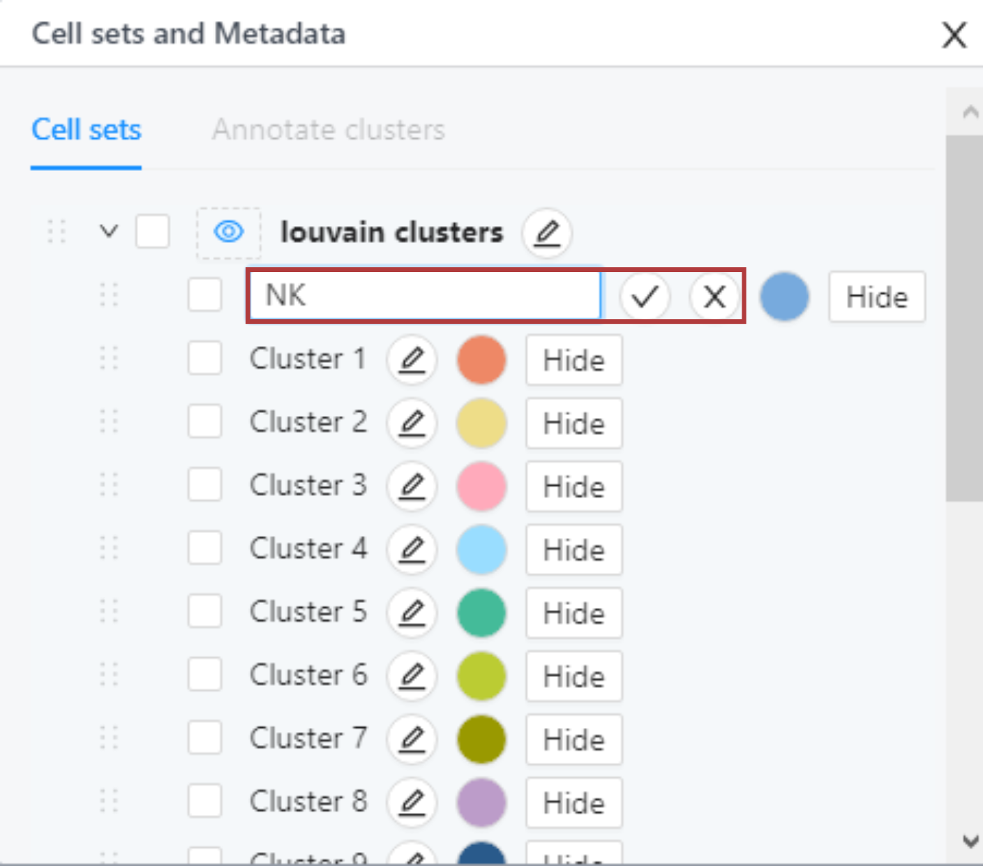
To change the name click the edit button next to the cluster name. After inputting the new name, click the checkmark to save the name or the cross to cancel. Any changes to cluster names made in this tile propagate all other modules of the platform.

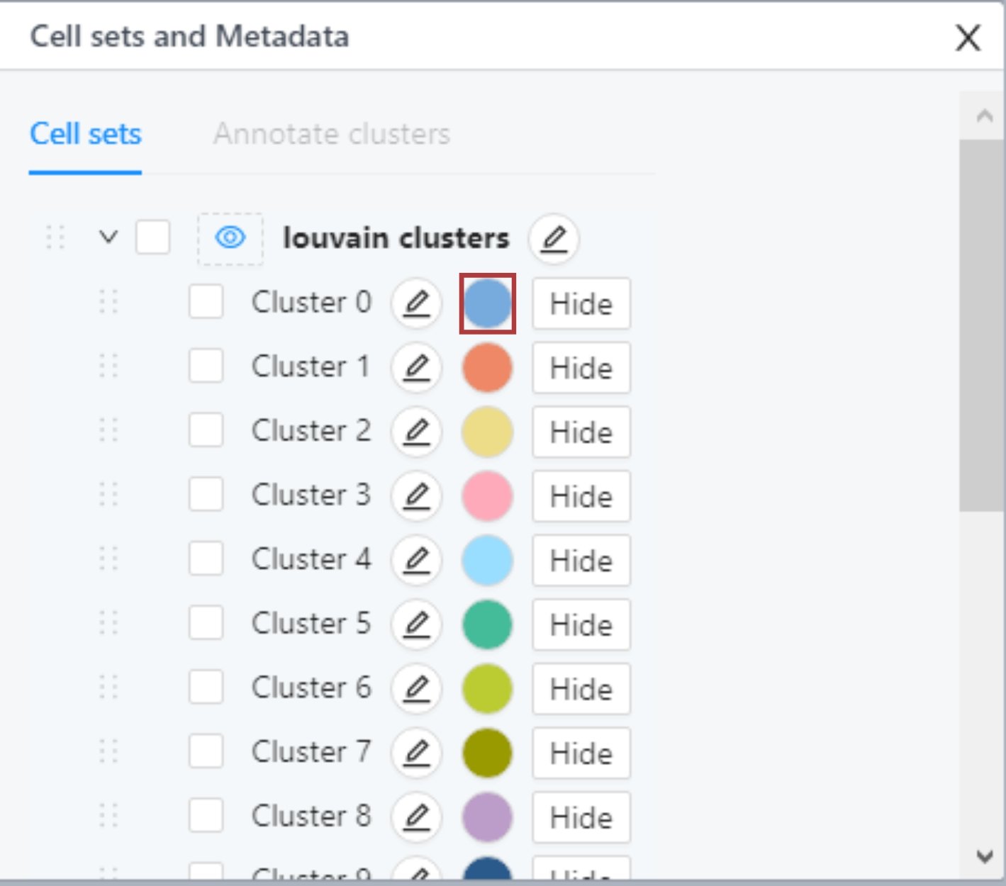
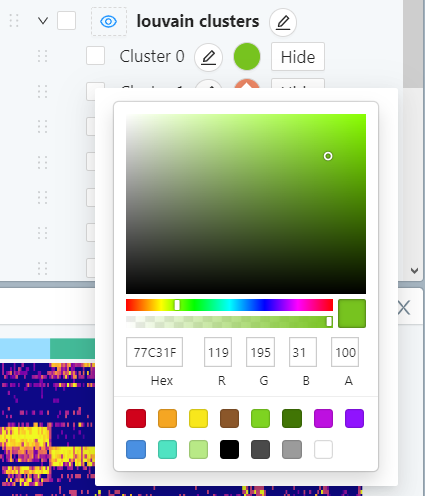
To change the color of a cluster, click on the colored circle next to the cluster. In the popup, choose the new color and it will be applied automatically. Any changes to cluster colors made in this tile propagate all other modules of the platform.
Changing names and colors of metadata tracks
You can also edit the names of samples or any added metadata tracks (such as “Tissue”). To change the name click the edit button next to the metadata track. After inputting the new name, click the checkmark to save the name or the cross to cancel. Any changes to sample or metadata track names made in this tile propagate all other modules of the platform.


You can also edit the names and colors of individual samples or metadata groups within the metadata tracks. To change the name click the edit button next to the item. After inputting the new name, click the checkmark to save the name or the cross to cancel. Any changes to sample or metadata names made in this tile propagate all other modules of the platform.


To change the color of a metadata item, click on the colored circle next to the item. In the popup, choose the new color and it’s going to be applied automatically. Any changes to sample or metadata colors made in this tile propagate all other modules of the platform.


Reordering clusters
It’s possible to rearrange the order of clusters. To reorder clusters, drag them to the desired position using the button (3 lines) on the left of the cluster name. The new order of clusters in the Cell sets and Metadata block will be then represented in the heatmap in the Data Exploration module, as well as all plots in the Plots and Tables module. See the example below.


Creating custom cell sets
Creating custom cell sets using a selection tool in the UMAP
New cell sets can be created using the lasso or rectangular selection tools that are available in the UMAP (or t-SNE) embedding plot. The lasso tool allows for a more precise selection than the rectangle selection tool.


In the popup, name the new cluster and click on the save button.

The new cluster will appear in the ‘Custom cell sets’ list in the Cell sets and Metadata tile. To see the new cell set colored in UMAP, click on the eye icon next to ‘Custom cell sets’.

Custom cell sets based on gene expression
You may want to create a new custom cell set based on the expression (or lack of expression) of one or more genes. In the gene list on the right-hand side of the Data Exploration module, you can select one or more genes of interest using the checkboxes next to the genes.


Then click the 'Cellset' button to generate a new cell set based on the expression of the selected genes.

You can then set the thresholds of expression for each selected gene in the modal. For example, you can select only the cells that express a particular gene at very high levels; or you can select only the cells that lack expression of selected genes. Then click ‘Create’.

When you click 'Create', your new cell set will appear in the Custom cell sets list in the Cell sets and Metadata tile. To see the new cell set colored in UMAP, click on the eye icon next to ‘Custom cell sets’.

Custom cell sets of combined Louvain clusters
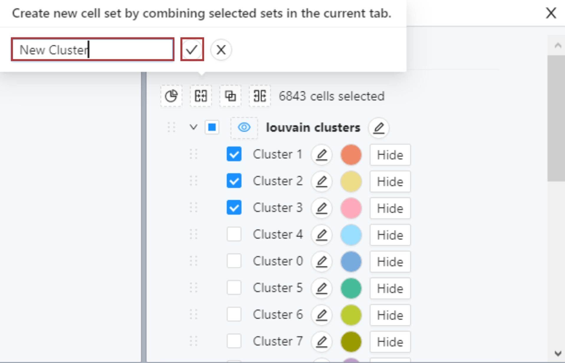
Locate the list of Louvain clusters in the Cell sets and Metadata tile. Select two or more clusters that you would like to combine using the checkboxes next to cluster names.

Then click the ‘Combine’ button.

In the popup, name the new cluster and click on the save button.
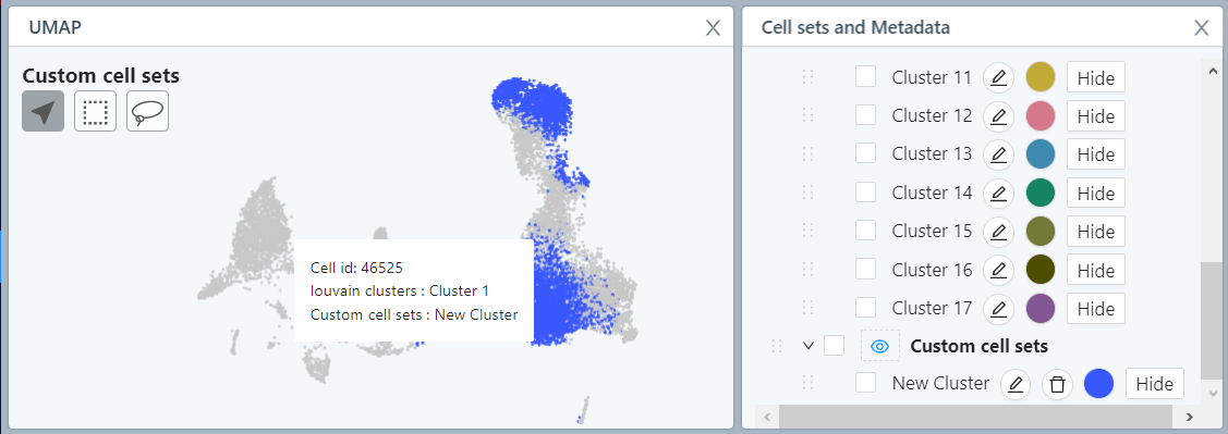
The new cluster will appear in the ‘Custom cell sets’ list. To see the new cell set colored in UMAP, click on the eye icon next to ‘Custom cell sets’.
Note that if you want to copy over all your other Louvain clusters to the Custom cell sets list, you can do so using the 'Combine' button with only one cluster selected at a time. This essentially copies the Louvain cluster to the Custom cell sets list.
Intersect selected clusters
Intersecting selected cell sets can be very useful when working with non-mutually exclusive cell sets. For example, you’ve created two new cell sets based on gene expression. Cell set 1 contains cells with gene expression of Gene 1 greater than 0.10, and cell set 2 contains cells with gene expression of Gene 2 less than 1. Now, there might be some cells in both of these new cell sets that are the same - with gene expression of Gene 1 greater than 0.1 and Gene 2 less than 1. Intersecting cell set 1 and cell set 2 will highlight cells present in both cell sets and combine them in a new cluster.
To use this function, locate the list of Louvain clusters in the Cell sets and Metadata tile. To create an intersection of cells, select clusters using the checkboxes next to cluster names.

Then click the ‘Intersection’ button.

In the popup, name the new cluster and click on the save button.

The new cluster will appear in the ‘Custom cell sets’ list. To see the new cell set colored in the UMAP embedding, click on the eye icon next to ‘Custom cell sets’, and hide clusters that you don’t want to see on the UMAP.

Create a new custom cell set from the complement of selected clusters
Using this function, you can create a new custom cell set that contains all cells that are not in the selected cluster(s). This can be useful and time-saving when you have many clusters and want to create a cell set with all cells outside of these clusters.
For example, you’ve created three new cell sets based on gene expression. Cell set 1 contains cells with gene expression of Gene 1 greater than 1, cell set 2 contains cells with gene expression of Gene 2 greater than 1, and cell set 3 contains cells with gene expression of Gene 3 greater than 1. Creating a new cell set from the complement of these three aforementioned cell sets will result in a cluster of cells with gene expression of Gene 1, 2, and 3 greater than 1.
Look at the close-up of a UMAP visualization of the three cell sets created based on gene expression versus a complement of these three cell sets.


To use this function, locate the list of Louvain clusters in the Cell sets and Metadata tile. To create a cell set from the complement, select clusters using the checkboxes next to cluster names. You can select one or more clusters.

Then click the ‘Complement’ button.

In the popup, name the new cluster and click on the save button.

The new cluster will appear in the ‘Custom cell sets’ list. To see the new cell set colored in the UMAP, click on the eye icon next to ‘Custom cell sets’ and hide custom clusters that you don’t want to see on the UMAP.

Subset selected cell sets to a new project
You can create a new project by subsetting a cell selection from your project. This allows for a further deep dive into part of your data, or for removal of contamination from your project.
When you have made a selection of a group of cells, a subset button appears in the Cell sets and Metadata tile.

When you click on the subset button, a pop-up appears to start a new project from your current cell selection. You can change the name of the new project, if you wish. Then click ‘Create’, to make a new project containing your selection.

Data Processing is run for this subset project, after which you can start your deep dive in the Data Exploration module for the subset of cells.


UMAP or t-SNE embedding tile
The tile on the top left of the Data Exploration module shows the embedding - UMAP or t-SNE - that was customized in step 7 of the Data Processing module. UMAP is shown by default. To change between UMAP and t-SNE, go back to step 7 of Data Processing to change your selection. The embedding plot in the Data Exploration module is interactive, allowing you to zoom in and out to focus on a particular area of interest, move, and hover over single cells. Hovering over a single cell gives you information about the cell ID and the cluster the cell belongs to, with the selected cell simultaneously highlighted in the marker heatmap.

The embedding is colored by Louvain clusters by default. To find out how to color the embedding plot using other parameters, go to the Coloring the UMAP embedding section. The colors of clusters can also be changed; more in the Changing names and colors of clusters section.
The UMAP plot also allows the creation of new custom cell sets by using the lasso or rectangular selection tools. Read about how to use the selection tools in the Creating custom cell sets using a selection tool in the UMAP section.

Coloring the UMAP embedding
In the Data Exploration module, the embedding plot (UMAP or t-SNE) is colored by Louvain clusters by default. To change the coloring of the embedding plot, use the "eye” icons that are located throughout this module. Several examples are shown below.
To color the embedding plot with the expression of a specific gene, select the eye icon next to the gene name in the gene list.

To color the embedding plot by custom cell sets, click on the eye icon next to ‘Custom cell sets’ in the Cell sets and Metadata tile. Unselected cells are colored gray.

You can also color the embedding by sample or metadata by clicking on the eye icon. Click on the eye icon next to ‘Samples’ to view the embedding colored by samples.

You can hide one or more clusters, samples, or metadata groups from the embedding plot and heatmap.
To hide a particular cluster from the embedding plot and heatmap, click the Hide button on the right side of the cluster name in the Cell sets and Metadata tile. To unhide a cluster or clusters, click the ‘Unhide’ button or use ‘Unhide all’ to unhide all hidden clusters. Metadata groups and Samples can also be hidden/unhidden in this way.

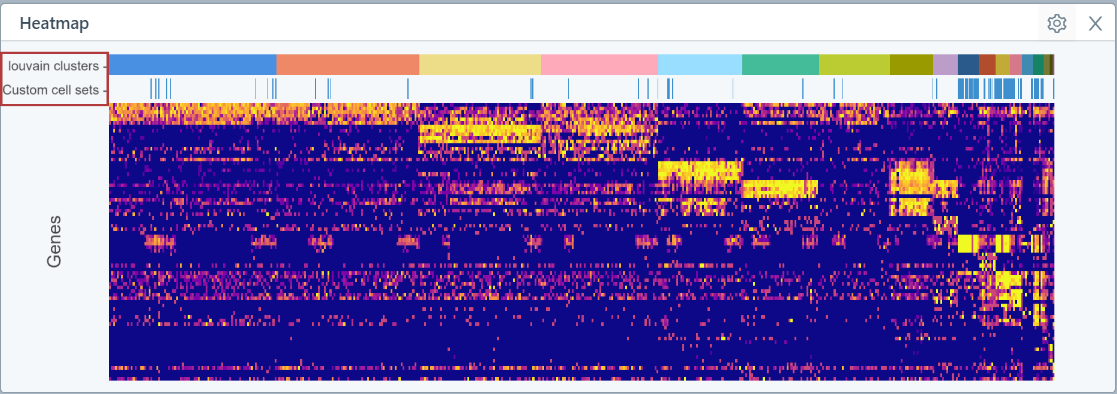
Heatmap
The heatmap shows marker genes for the Louvain clusters by default. The number of genes shown per cluster varies depending on how many clusters you have in your dataset. You can zoom in on a specific cell set of interest in the heatmap, and hover over marker genes to identify the gene name which will help to identify the represented cell type.


The heatmap settings menu is accessed by clicking on the gear/cog icon. In this menu, you can add sample/metadata tracks to the heatmap view or reorder the heatmap, as explained below.

Adding sample/metadata track to the heatmap view
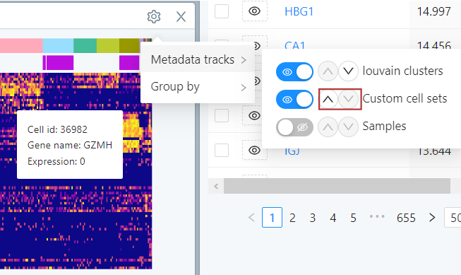
To add sample or metadata tracks to the heatmap view, hover over Metadata tracks in the heatmap settings menu. In the sub-menu, toggle the eye icon to add a metadata track. The toggled selections appear as colored tracks above the heatmap view.


Reordering the heatmap
Reordering metadata tracks
Selected cluster/sample/metadata tracks (see the previous section) appear as colored tracks above the heatmap. To change the order of these tracks, click on the arrow icon in the ‘Metadata tracks’ sub-menu to move the track up or down in the plot view.
The item on top of the list is also going to be shown at the top of the heatmap tile. Note that this doesn’t reorder the cells within the heatmap itself - this is done using the ‘Group by’ function (see the next section).

Group by a parameter
To reorder the cells viewed in the heatmap, hover over ‘Group by’ in the settings menu. In the sub-menu, hover over ‘Select the parameters to group by’ dropdown menu. Click + to add a parameter you want to order cells by. To exclude a parameter, click - on the left of the parameter.

Then, in the ‘Group by’ sub-menu, arrange the parameters in descending order by which you would like to group them by.
In the example below, the heatmap is ordered first by sample and then by Louvain clusters:


Viewing genes in the heatmap
You can search for specific genes of interest in the gene list. If you want to look at these genes in the heatmap, you can select them using the checkbox and click ‘Heatmap’.

This gives you an option to add or remove the selected genes from the heatmap or overwrite the heatmap with the selected genes(s).

Clicking remove will remove the selected gene(s) from the heatmap. Clicking add will add the selected gene(s) to the heatmap.
Using overwrite, the heatmap only shows the expression of the selected gene(s). If at any point you want to re-load the default heatmap view showing marker genes, simply reload the page.

Gene list
You can find the full Gene list for your dataset in the ‘Genes’ tile on the right-hand side of the Data Exploration module. By default, genes are presented in descending order by dispersion. Dispersion describes how much the variance deviates from the mean. Genes with high dispersion have a high level of variation between cells in the dataset.
Rearranging the gene list
You can rearrange the gene list based on the gene name or dispersion by clicking on the column names (Gene and Dispersion). Both ascending and descending options are available to view.


You will see a change in the up and down triangle symbol next to Gene or Dispersion when you reorder the gene list.

Ascending (triangle pointing upwards)

Descending (triangle pointing downwards)
Search for genes in the gene list
You can search for genes that contain, start with or end with certain letter/s or possible subunits. Your search is applied automatically to the gene list as you type.
For example, select option ‘contains’ and input ‘HB’ in the search box.

Or you can select the option ‘starts with’ or ‘ends with.’ For example, input ‘Z’ in the search box.


To clear a gene search, delete your input in the search box or click the cross button (✖) on the left of the search box.
Viewing gene information
If you want to view information on a particular gene in the Gene List, click on the gene name.

This action opens a new window showing the selected gene in GeneCards.

Note that the GeneCards database is used primarily for human genes and may not provide useful information if your dataset is from a species other than human.
Differential expression analysis
Differential expression analysis allows you to determine which genes are expressed at different levels between experimental groups. Differentially expressed genes can then be used in pathway analysis to offer insight into the biological processes affected by the condition of interest.
Using Cellenics®, you can find the differential expressed genes between two groups of cells, where each group must have at least 3 cells. Differential expression can be calculated using the differential expression tab on the right side in the ‘Genes’ block.
You can compare cell sets within a sample/group, which allows you to find marker genes that distinguish clusters from one another.
Alternatively, you can compare a selected cell set between samples/groups to find genes that are differentially expressed between two experimental groups.
Compare cell sets within a sample/group
The differential expression calculation to compare cell sets within a sample or group uses the presto implementation of the Wilcoxon rank sum test and auROC analysis. For more information see the presto vignette.
To perform this analysis, choose a cell set you want to compare in the first drop-down menu (1). Choose another cell set, the option ‘Rest of Louvain clusters’ or ‘All other cells’ in the second drop-down menu (2). [Note that in the case of Louvain clusters, ‘Rest of Louvain clusters’ and ‘All other cells’ is the same because all cells are assigned to a Louvain cluster; whereas for Custom cell sets, these two options will be different if not all cells in the dataset are assigned to a Custom cell set.] Lastly, select the sample/group within which you want to compare cell sets or choose the option ‘All’ (3).
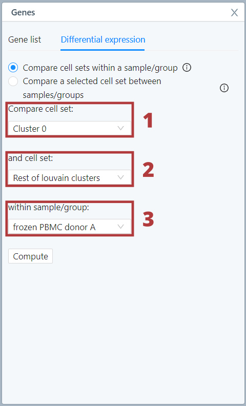
Then click compute.

You will be presented with the differential expression (DE) results table: a list of genes in descending order of log fold change (logFC). The table returns the following results:
LogFC: The fold change is the ratio of the expression of a gene between the two groups being compared. They are then log-transformed. Genes with a positive logFC that appear at the top of the list are expressed at higher levels in the comparison group A compared to group B. Given that logFC = log2(A) - log2(B), if log2(A) is negative and log2(B) is positive, then the logFC will be positive.
Adj p-value: The probability of observing the difference in expression for a given gene under the assumption that said gene is not differentially expressed. In addition, the value is adjusted using the Benjamini–Hochberg correction for multiple hypothesis testing, to account for the fact that when testing thousands of genes, some might have a small p-value due to random chance. The smaller it is, the higher the chance the gene is actually differentially expressed.
Pct1: The percentage of cells where the gene is expressed in the first group (A).
Pct2: The percentage of cells where the gene is expressed in the second group (B).
AUC: Area under the receiver operating characteristic (ROC) curve. It is proportional to the Wilcoxon U statistic calculated by the rank-sum test. The larger it is, the more likely it is that the corresponding gene is differentially expressed.

The DE gene list can be re-ordered in the table by other calculated parameters - adjusted p-value, PCT 1 (the percentage of cells where the feature is detected in the first group), PCT 2 (the percentage of cells where the feature is detected in the second group), and AUC (area under the receiver operating characteristic curve). Both ascending and descending options are available to view.
Clicking on ‘Show settings’ will show your chosen cell sets and samples/groups that have been compared in this DE calculation.

Note that to download the DE results, you must visit the Volcano plot in the Plots and Tables module. Unfortunately, the DE results table cannot be downloaded from the Data Exploration module.
Compare a selected cell set between samples/groups
The differential expression comparison of a selected cell set between samples or groups uses a pseudobulk limma-voom workflow. This is considered best practice for between sample comparisons. Pseudo-bulk differential expression sums the counts for all cells within a cluster for each sample and then uses standard differential expression methods designed for bulk RNA-seq. One major benefit to doing this is that it treats the sample as the level of replication, instead of falsely assuming that each cell is independent.
To perform this DE analysis, choose a cell set you want to compare in the first drop-down menu (1). Choose the first sample/group to compare in the second drop-down menu (2). Lastly, select the second sample/group you want to compare with the first sample/group or choose the option ‘Rest of Samples’ or ‘All other cells’ (3).

Note that in some comparison selections, this warning message will appear:

The message explains that in your selected comparison, there are fewer than 3 samples with the minimum number of cells that’s required to perform the DE calculation. The most likely explanation is that you are comparing 1 sample to 1 other sample. An alternative explanation is that you are comparing 3 or more samples, but that there are too few cells (<10) in one or more of the comparison groups, which is resulting in only 2 ‘valid’ comparison groups that contain enough cells to perform the DE calculation.
In this case, you can still go ahead and perform the DE calculation, but the DE results table will only display the list of DE genes and logFC value. No adjusted p-value will be calculated as it is not considered statistically sound to calculate such a p-value on a 1 versus 1 comparison.
When you have made your selections for the DE calculation parameters, click ‘Compute’.

You will be presented with the differential expression (DE) results table: a list of genes in descending order of log foldfull change (logFC).
The table returns the following results:
If the comparison contains 3 or more samples (e.g. 2 control vs 1 treated) then the DE results table presents both the logFC and the adj p-value. In this case, the p-values generated from pseudo-bulk comparisons are statistically accurate and can be used to determine biological significance.
For 1 vs 1 comparisons (e.g. 1 control vs 1 treated), only the logFC is returned in the results table, because p-values are not appropriate with this small N. LogFC estimates can be used to ascertain the magnitude of the difference between the two samples but not to draw any statistical inferences.
The gene list can be reordered in the table by other calculated parameters by clicking on the column titles.

Clicking on ‘Show settings’ will show your chosen cell sets and samples/groups that have been compared.
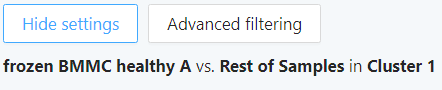
Advanced filtering
To filter the DE gene list, click ‘Advanced filtering’.

In the popup menu, you can select advanced filtering options. There are three pre-set filtering options which allow you to quickly filter for only the up-regulated genes (with a positive logFC), only the down-regulated genes (with a negative logFC) or only the significant genes (with an adjusted p-value of <0.05):


Alternatively, you can add your own custom filter using the ‘Add custom filter’ option. Here, you can select to filter by any of the DE results parameters and set a filtering threshold of your choice.
Pathway enrichment analysis
Pathway analysis identifies biological pathways that are enriched in the differentially expressed gene list more than would be expected by chance. The goal is to give the list of genes across different phenotypes a biological context by condenscing down a potentially long list of genes into a few select biological pathways.
Click ‘Pathway analysis’ after performing differential expression, to start your pathway analysis. We strongly recommend using Advanced filtering to filter your list of DE genes before performing pathway analysis. This is because the list of differentially expressed genes is very long and contains both up- and down-regulated genes with varying levels of significance. So, further filtering will lead to more consistent and clear pathway analysis results.
Once your list of DE genes has been filtered using the ‘Advanced filtering’ tool, select ‘Pathway analysis’ to begin:

Pathway analysis can be performed on a list of differentially expressed genes using the external service providers PantherDB or Enrichr. The list of genes and species will be submitted to the external service, and no other information will be sent.
We recommend running your pathway analysis using both PantherDB and Enricher and then comparing the results. Your final choice for the pathway analysis service might depend on the databases in the platforms, user interface, and, ultimately, on your personal preference.
For help using these external pathway analysis services, we recommend visiting the Help pages for PantherDB and Enrichr.
PantherDB
Select the ‘pantherdb’ toggle at the top of the pathway analysis modal:

In the pathway analysis modal, you can confirm the species of your dataset. You can also select the number of differentially expressed genes that will be included in the pathway analysis by clicking ‘Top’ and inputting the desired number. To send all the genes in your filtered list, select ‘All’.

Then, initiate your pathway analysis by clicking ‘Launch’.

PantherDB is hosted on an unsecured server (HTTP), so you will see a warning upon launch. Click “Send anyway” to continue. The list of genes and species will be submitted to the external service, and no other information will be sent. See the example below.

You will be redirected to the PantherDB website in a new tab.

We recommend inputting the reference list of genes by setting it in "Reference List" on the PantherDB results page and re-run the pathway analysis. If gene names in Cellenics® are different than in the reference list of genes on PantherDB (for instance, lowercase vs. uppercase gene names), the results of pathway analysis will be incorrect.
For further help using PantherDB, please visit the relevant help pages on the PantherDB website: http://pantherdb.org/help/PANTHERhelp.jsp.
Enrichr
Select ‘enrichr’ at the top of the pathway analysis modal.
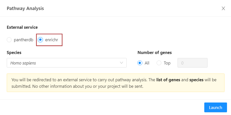
In the pathway analysis modal, you can confirm the species of your dataset. You can also select the number of differentially expressed genes that will be included in the pathway analysis by clicking ‘Top’ and inputting the desired number. To send all the genes in your filtered list, select ‘All’.
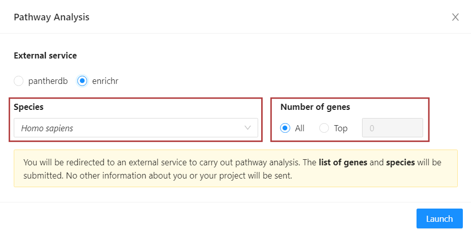
Then, initiate your pathway analysis by clicking ‘Launch’.

You will be redirected to the maayanlab.cloud Enrichr page in a new tab.
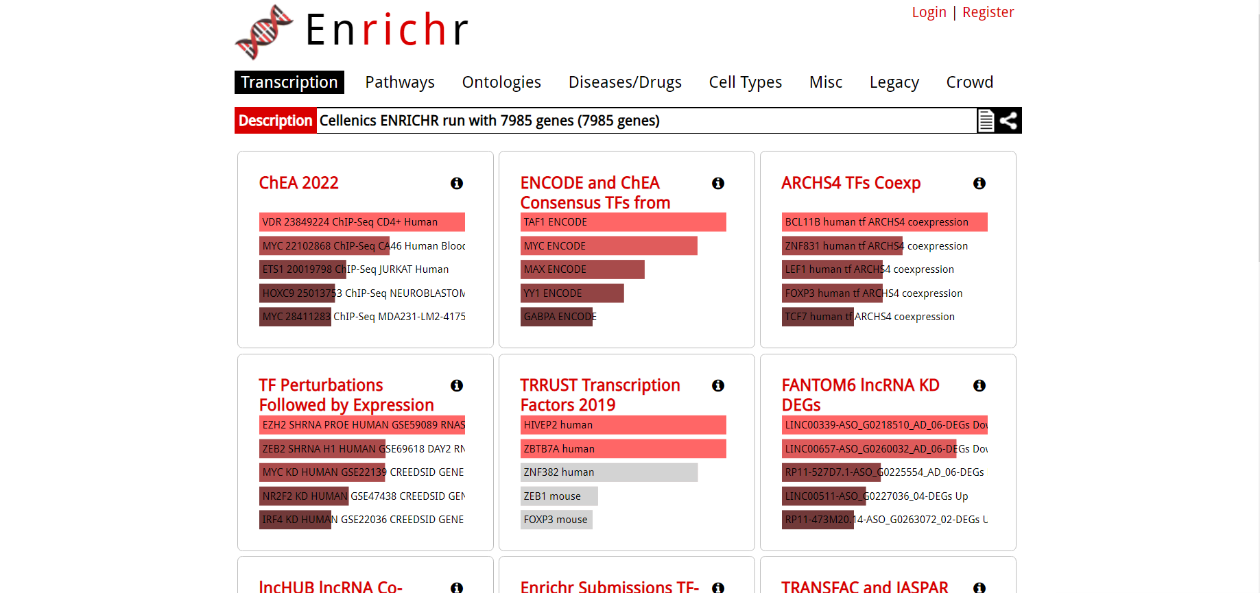

For further help using the Enrichr pathway analysis tool, please visit the relevant help pages on the Enrichr website: https://maayanlab.cloud/Enrichr/help.
Plots and Tables
Overview
The Plots and Tables module of Cellenics® provides a wide range of pre-loaded data visualization options to quickly and easily get insights from your data. It also allows users to customize the plots and export them in a variety of formats.
The module is organized into three sections to make finding the right plot easy and intuitive. The Cell sets & metadata section contains plots that graphically represent cell set properties - categorical embedding, frequency plot, and a trajectory plot. The Gene expression section contains plots that represent the expression of individual genes across cell sets, such as violin plots, dot plots, and more. The Differential expression section includes a volcano plot that visually represents differences between and within groups.

General options
All the plots have general customization options!

Main schema
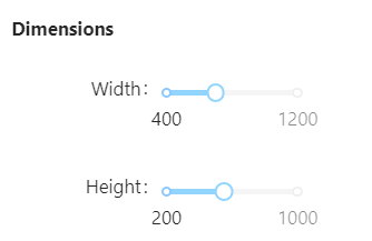
Under the main schema control, you can change the dimensions of the plot - customize the plot’s height and width using the slider scale.
In the title section, you can define the plot's title, change the title's font size, and indicate the location of the title.


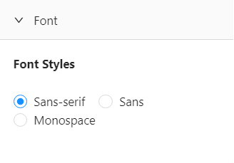
In the font section, you can change the text font in the plot from Sans Serif to Sans or Monospace.


Axes and margins
Under the Axes and margins control, you can customize the y-axis and x-axis. You can also customize the margins and grid lines.

You can change the titles of the x- and y-axis, as well as the size of the axis titles, using the slider. Just slide the dot to your preferred value. The changes to axes titles will be applied to the plot automatically.


You can also rotate the labels on the x-axis. To do this, toggle the “Rotate X-Axis Labels” button.

You can change the size of axes labels using a slider scale. Just slide the dot to your preferred value.


To change the margins in the plot, use the slider scale to change the margins from 0 to your preferred value. This will move the plot off-center by offsetting automatic margins.

To add grid lines to the plot, use the slider scale to change the grid line weight from 0 to your preferred value.

In this section, you can also override the automatic axes ranges.
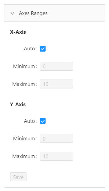
To manually input values for axes ranges, deselect the Auto control under X-axis and/or Y-axis. Then input your preferred minimum and maximum values, and click Save.


Color inversion
The Colour inversion control allows inverting the color of the background. If the standard color of the plot's background is white, this control enables you to turn the background black.


Markers
This section applies to embedding and volcano plots. Here, you can change the style and shape of markers.

The point (marker dot) size can be changed from 1 to 100 using a slider scale.


Point opacity can also be changed using a slider scale for the embeddings. The default opacity is at 5, but it can be customized on a scale from 1 to 10.


There are two options for point shape - diamond and round. To change the shape, select your preferred point shape.


Legend
Under Legend control, you can decide whether to show or hide the plot legend. To hide the legend, toggle the Hide option.
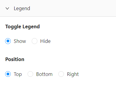


You can also choose the position of the legend by clicking Top, Bottom, or Right.


Labels
The label control applies to the categorical and continuous embedding plots. You can use this control to show or hide the cell set labels.


You can also change the size of the labels if you choose to show them on the plot. This might be particularly helpful if you have a lot of clusters in the embedding and their names overlap. To change the size, use the size slider to choose your preferred value.


Additionally, in the volcano plot, you can find a control called “Add labels.” This option allows specifying the negative log10 of the adjusted p-value. Above your chosen values, labels for upregulated and downregulated genes will be displayed.

For example, here is a comparison of volcano plots where the gene labels are displayed above -log10 p-value of 100 versus -log10 p-value of 280.


Reset plots
All the plots have a reset button that appears after you make any changes to the default plot.
Click the blue reset button on top of the plot to return to the default plot and undo all changes.


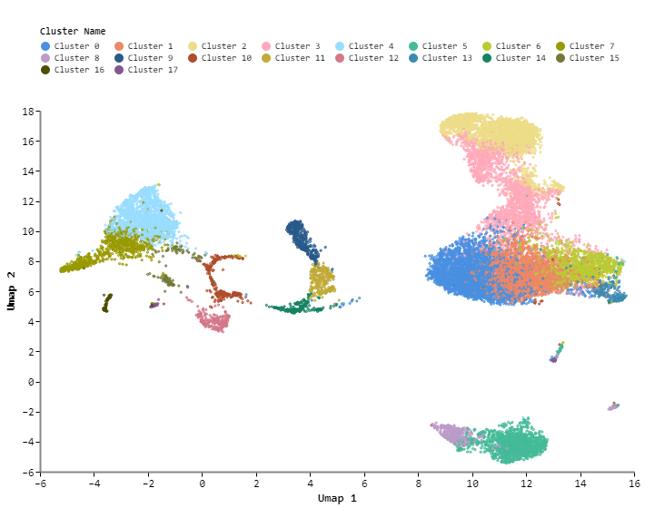
Cell sets & metadata
Categorical Embedding
The default categorical embedding plot shows a UMAP embedding of cells from all samples clustered and colored according to the Louvain clustering algorithm. You can read more about how this plot is generated in Step 7: Configure embedding section.
Categorical embedding allows the coloring of the UMAP according to categorical variables. These variables are discrete and used to split data based on specific characteristics, such as samples. The default embedding plot displays Louvain clusters.

Group by
You can use the Group by control to change the cell set category by which you would like to group cells.


Here is a UMAP plot grouped by custom cell sets.

And here is a UMAP plot grouped by samples. This plot shows the distribution of samples across clusters in the embedding.

Select data
Using Select data control, you can select a sample of interest. This will result in the embedding only showing cells from the selected sample instead of all samples.

For example, here is a categorical embedding plot of one sample - frozen PBMC donor A.

Frequency Plot
A frequency plot shows the distributional information of a variable. Simply, it summarizes the data by plotting how frequently a specific value occurs. In Cellenics®, the default frequency plot shows the proportions of cells from each cluster in every sample. So, the y-axis represents the proportions, which are frequency values. While the x-axis represents samples by which the cells are grouped. You can use a frequency plot to see if there is a significant shift in the proportions of cells between samples.

Select data
You can change the metadata and cell sets used for this plot using select data control. If you have multiple metadata tracks, you can change the variables represented by the x-axis. Then you can change the cell set whose frequency you want to plot in the metadata intervals.
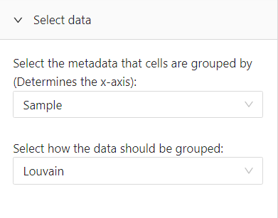
For example, you can change the cell set from Louvain clusters to Custom cell sets.
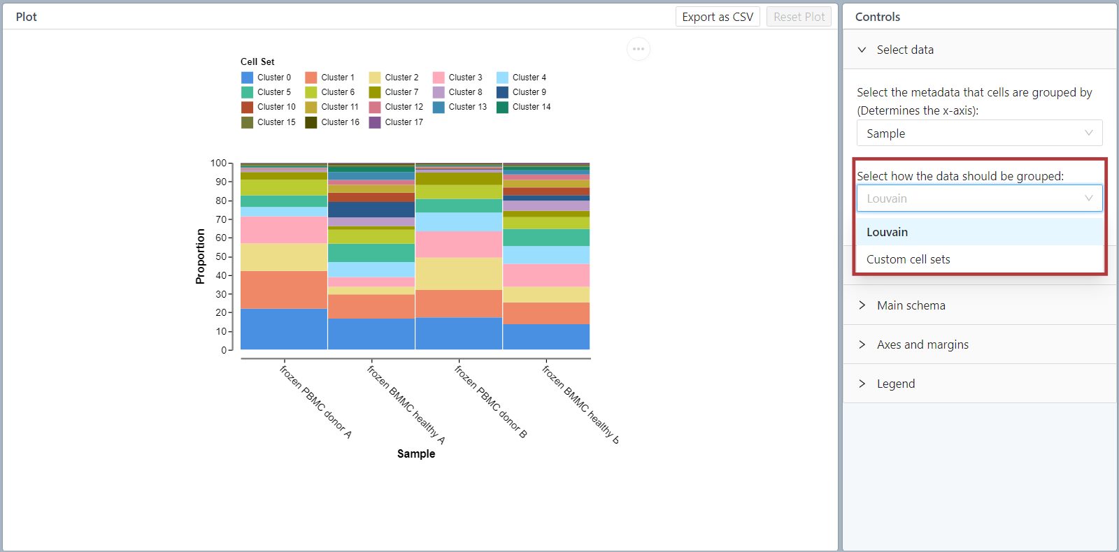

Plot type
You can change the plot type to a frequency plot of absolute counts. To do this, use the Plot type control and click on Count. Absolute counts reflect the number of cells in that cluster in a sample, while proportions reflect the proportion of cells in the cluster compared to all other clusters.


Trajectory Analysis
Trajectory analysis allows the user to determine a pattern of a dynamic biological process experienced by cells - a "trajectory" of gene expression changes. Then the cells are arranged according to their progression through that process, which means they are placed at their proper position in the trajectory. This progression can be quantitatively measured using pseudotime. Pseudotime has been defined as “an abstract unit of progress: simply the distance between a cell and the start of the trajectory, measured along the shortest path.” [1].
Calculate root nodes
To get started, select cell sets to use for trajectory analysis. By default, all Louvain clusters are included. However, you can choose to perform trajectory analysis for specific clusters, samples, or metadata. Click on the box above “Calculate root nodes”, and a drop-down menu will appear with all the cell sets in your dataset.


For example, the selection below includes all Louvain clusters and the PBMC donor sample. When you have made your selection, click “Calculate root nodes”.

Select root nodes
After the calculation is done, select root nodes by clicking on the white points. The root nodes signify where you want the trajectory to start. You can select multiple nodes at once by drawing a selection. Hold down the Shift key to do this, and then click and drag. Nodes inside the selection will be added as root nodes.

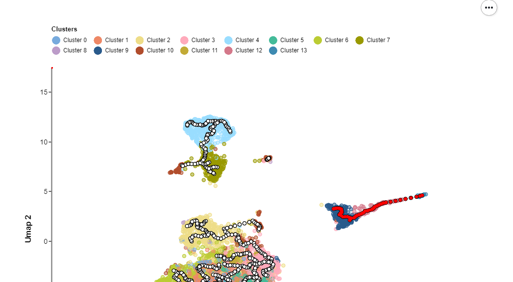
Deselect nodes by clicking on a selected node or by clicking Clear selection.
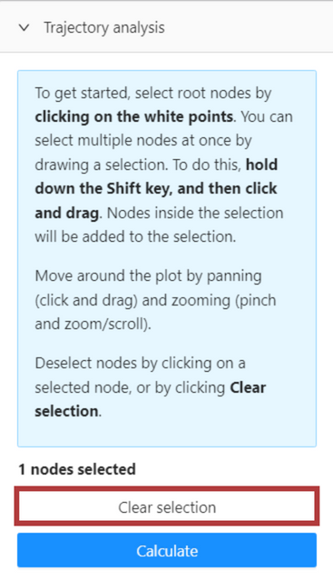
When you have made your selection, click calculate. The trajectory plot will be colored by pseudotime. Move around the plot by panning (click and drag) and zooming (pinch and zoom/scroll).

If you have made changes to your selection (e.g., cleared the selection or added new nodes to the selection) after clicking calculate, you can recalculate the pseudotime.

Here is an example of a trajectory plot from our article “Reproducing a published trajectory analysis plot with Cellenics®.”

Display
Under the display control, you can change plot values from pseudotime to cell sets. Before selecting root nodes and calculating pseudotime, the default plot values will be based on cell sets.

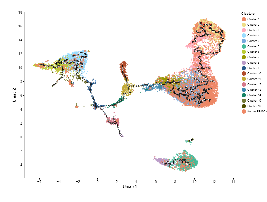


You can also hide the starting nodes (white points) from the plot.


Gene expression
Continuous Embedding
The continuous embedding plot allows you to see the expression of a particular gene across the Louvain clusters.
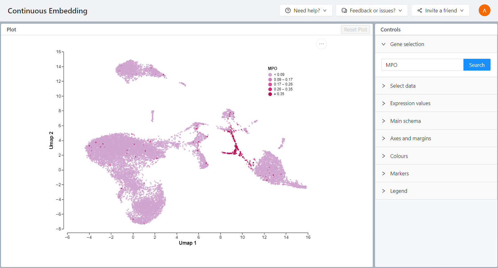
Gene selection
Type the gene name in the search box to select a gene of interest. You can find the search box under the Gene selection control.


Select data
You can also select the data to view on the embedding. For example, you can choose to see the gene expression in cells from a specific sample. To do this, use the Select data control. Below is an example of HBA1 gene expression in a frozen BMMC healthy B sample.


Expression values
You can choose to have capped or uncapped values under the “Expression values” control, where the default is set to capped Capped values for the expression level of a gene in a given cell refer to genes that are expressed at a level above a predetermined threshold, determined by the 95th percentile. These genes are said to be capped because their expression values are artificially set to this threshold, even though their true expression level may be higher.
Whereas uncapped values refer to genes that are reported as their actual expression value.
Capping can be done to manage the potential high variability often found in scRNA-seq data. By capping the expression values at this threshold, one can mitigate the impact of extremely high outliers which may not be biologically relevant but rather artefacts or noise. However, a limitation of this approach is that it could potentially result in the loss of meaningful information about genes that are naturally expressed at extremely high levels or in specific cellular conditions.
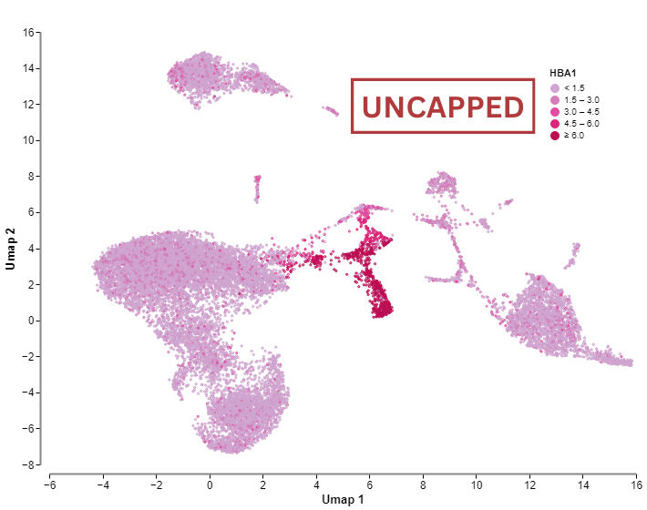

Heatmap
The heatmap shows marker genes for the Louvain clusters by default. You can choose to see custom genes or marker genes in the heatmap.

Gene selection
By default, five marker genes per cluster are shown, the same as the default heatmap in Data Exploration. To select custom genes, type in a gene name and select it to add it to the plot. You will see automatic suggestions for the genes when you are typing out the gene name. Click on the gene in the suggestion box to add the gene, or click on the Add button. To add multiple genes, separate them with a space or comma.

The genes you have selected will appear below the search bar.

To rearrange the order of the genes on the y-axis, drag and drop these genes.


To deselect a gene click on the X on the right of the gene name.

To see the expression of marker genes:
Click on Marker genes.
Type the number of marker genes per cluster that you want to plot.
Click the Run button to plot the heatmap.


In Custom and Marker gene selection, you can also choose to show or hide gene labels.

Metadata tracks
To add metadata tracks, click on the Metadata tracks control. Toggle the eye icon to add a metadata track to the heatmap. The toggled selections appear as colored tracks above the heatmap.


To change the order of metadata tracks or Louvain cluster tracks in the heatmap, click on the arrow icon to move the track up or down in the plot. The item on top of the list will also be shown at the top of the heatmap block. Note that this doesn’t reorder the default ordering of cells as it’s still grouped by Louvain clusters. Cells can be reordered within the heatmap using the ‘Group by’ control (see the next section).


Group by
To reorder the cell ordering in the heatmap, click on the ‘Group by’ control. In the popup, hover over the ‘Select the parameters to group by’ drop-down menu. Click + to add a parameter you want to order cells by. To exclude the parameter, click - on the left of the parameter.


Then click on the up arrow to change the ordering of the cells. The parameter on the top of the list will be used as a grouping parameter. In the example below, the heatmap is grouped by Custom cell sets.
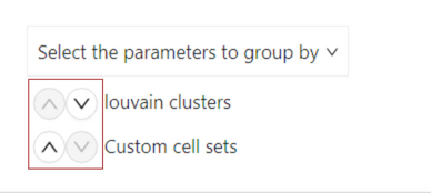


Expression values
You can change the type and capping of the expression values under the Expression values control. You can choose to use raw values or Z-scores. You can also choose to have capped or uncapped values. Capped values for the expression level of a gene in a given cell refer to genes that are expressed at a level below a predetermined threshold, typically set to be the detection limit of the scRNA-seq experiment. These genes are said to be capped because their expression values are artificially set to this threshold, even though their true expression level may be lower. Whereas uncapped values refer to genes that are reported as their actual expression value.

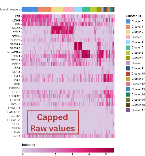


Violin Plot
The violin plot allows you to look at the distribution of normalized expression of a gene of interest across Louvain clusters by default. The black dots represent cells. Sometimes you can see black horizontal lines at the bottom of kernels. These are points that signify the cells where the gene is not expressed, and visually can look like a line on the plot.

Gene selection
Under the Gene selection control, you can select your gene of interest. Type the gene into the search box. You will see automatic suggestions of the gene when you are typing out the gene name. You can click on the suggested gene to autocomplete the gene name.
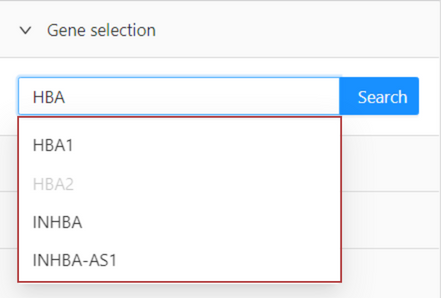
Click search to plot the violin plot.


View multiple plots
You can view multiple violin plots for the expression of different genes in a grid view in one window.
Type the gene name into the search box to plot multiple violin plots. You will see automatic suggestions of the gene when you are typing out the gene name. You can click on the suggested gene to autocomplete the gene name. To add multiple genes, separate them with a space or comma.

Click add to plot the expression of your selected genes. The selected genes are going to appear at the bottom of the section.


Note that the plots still need to be saved individually.
Drag and drop the genes in the gene list to rearrange the order of plots in the grid. To deselect a gene and remove a plot from the grid, click on the X on the right of the gene name.
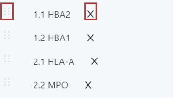
You can also change the dimensions of the grid. The grid dimensions are represented as Rows x Columns.
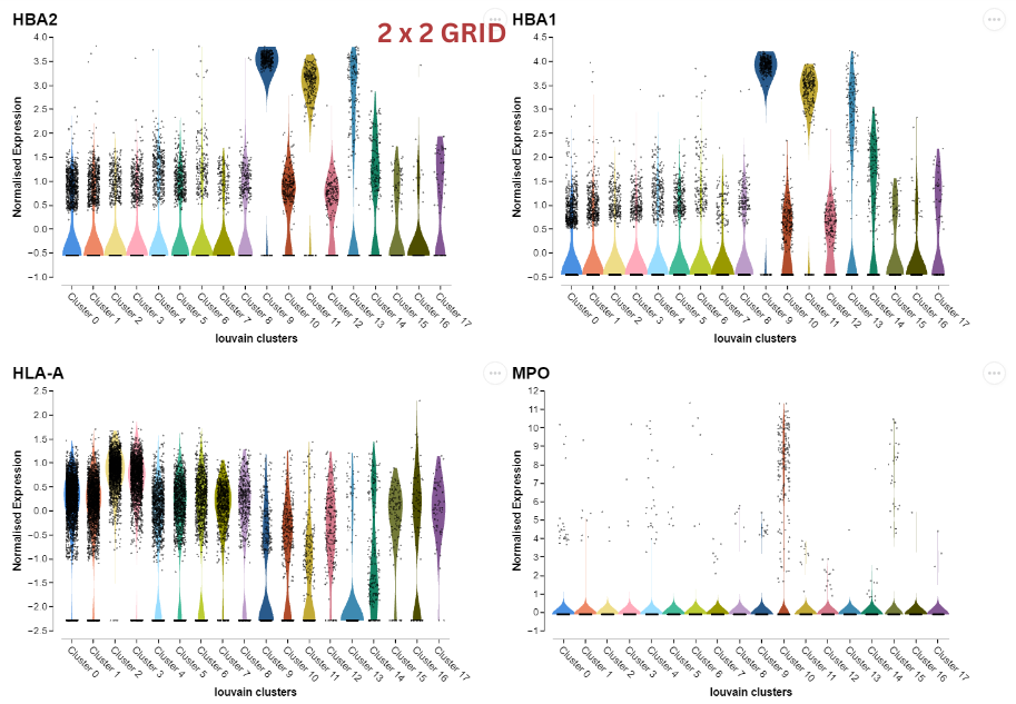

Under the same control, you can also find the options to select a specific plot and update the controls. If you have selected “Controls update: All plots”, then changes in other controls such as Select data and Data transformation are going to be applied to all the plots in the grid.

If you select a plot and choose “Controls update: Selected plot”, changes in controls are going to be applied only to the selected plot. For example, here the violin plot for the gene HBA2 is selected. And the controls are updated to apply only to this HBA2 violin plot.

For example, then increase the point size under “Markers” and the bandwidth under “Data transformation”. You can see that the HBA2 violin plot is now significantly different from the other plot in the grid.

Select data
You can change the metadata and cell sets used for this plot using select data control. If you have multiple metadata tracks, you can change the variables represented by the x-axis.


Then you can change the cell set or metadata to be used as data. The default option is to show ‘All’. However, you can choose to display only a part of the data. For example, group cells by Louvain clusters but only show data from a specific sample. To do so use the dropdown menu, and select the cell set/metadata you want to display.


Data transformation
Under the Data transformation control, you can change the type of gene expression values from normalized to raw values. Note the change in the values on the y-axis in the screenshots below.


You can also adjust the bandwidth, which impacts the density fit of the kernels. To change the bandwidth, move the slider to your preferred value. Values range from 0 to 1 in 0.05 intervals.


Dot Plot
In Cellenics®, the dot plot shows the percentage of cells expressing the genes of your choice. The percentage of gene expression in all the cells of a specific cluster is represented by the size of the dot. The smaller the dot, the smaller the percentage expression. If you see a bigger dot in a specific cluster, the gene is more expressed there. The color reflects the level of expression of the gene.
By default, three genes with the highest expression across all cells are shown.

Gene selection
You can look at the expression of custom genes of your choice or marker genes.
To select custom genes, type in a gene name in the gene search box. You will see automatic suggestions for the genes when you are typing out the gene name. To add multiple genes, separate them with a space or comma. Click Add to apply to plot your selected gene/s.


The gene/s you have selected will appear below the search bar.

To rearrange the order of the genes on the x-axis, drag and drop these genes in the gene list below the search box. To deselect a gene click on the X on the right of the gene name.

Click the Reset button at the bottom of the Gene selection control to revert to the suggested custom gene list.
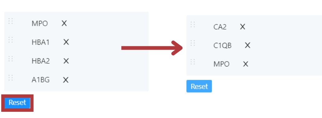
To see the expression of marker genes:
Click on Marker genes.
Type the number of marker genes per cluster that you want to plot.
Click Run to plot the marker gene dot plot.


Select data
In the dot plot, you can also change the cell sets or metadata that cells are grouped by, which determines the y-axis.
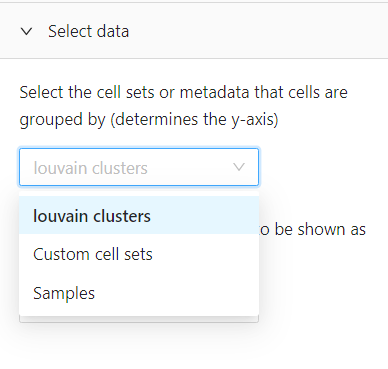
For example, you can look at the expression of your selected genes in your custom cell sets.


Or you could look at the expression of your selected genes in your samples.


You can also select the cell sets or metadata to be shown as data. For example, the cells can be grouped by Louvain clusters (y-axis), and you can select to view data only from one sample.


Size scale
You can also change the size scale of the dot plot. There are two available options - relative and absolute scale. Absolute scale will show total expression, while relative scale will be relative to what you select in the "Select data" control. So, if you select Louvain clusters, the size scale will be relative to all clusters, but if you select samples, the size scale will be relative to all samples.
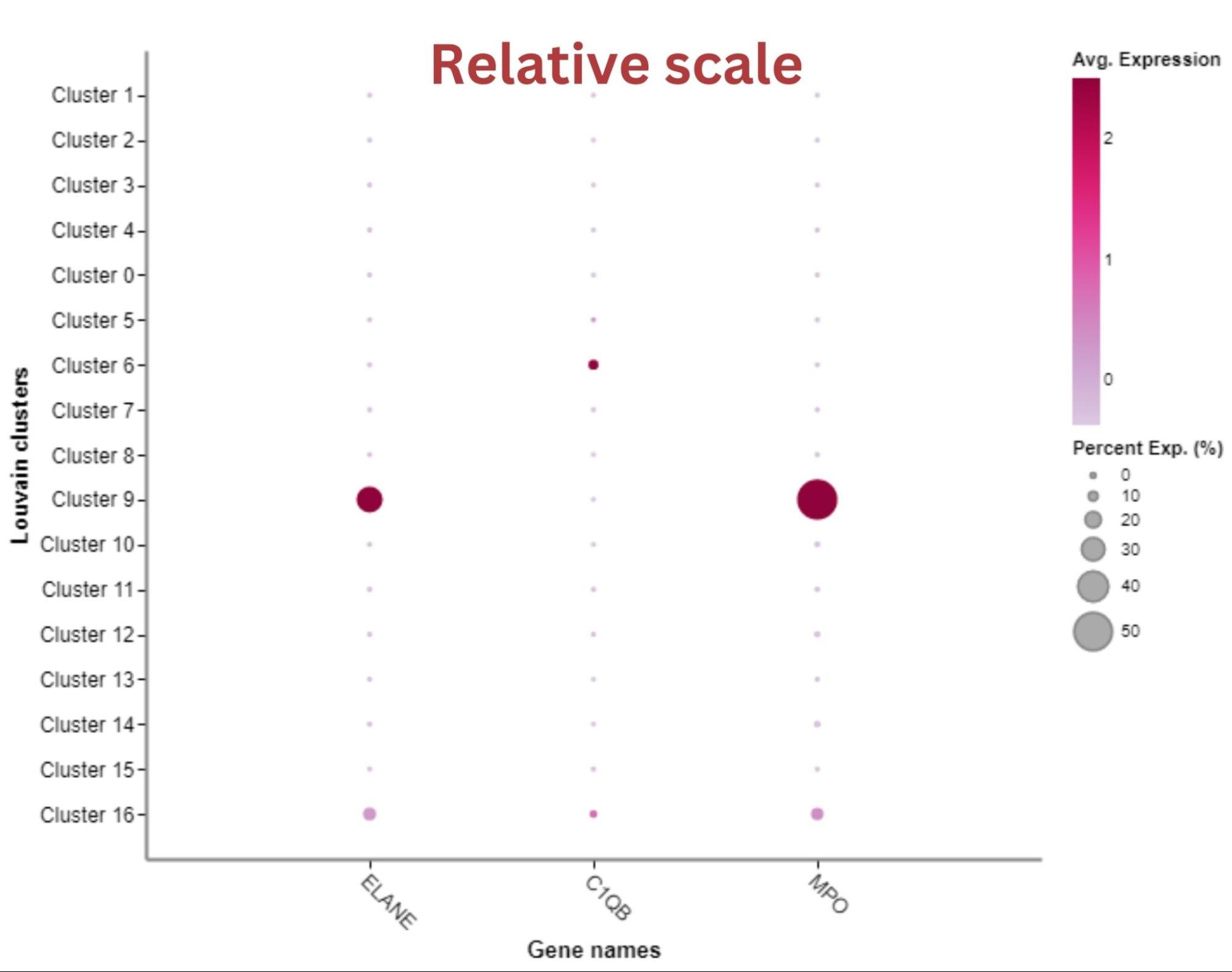

Normalized expression matrix
In the Plots and Tables module, you can download the normalized expression matrix for specific samples, metadata groups, clusters, and custom cell sets. The normalized expression matrix contains genes as rows and cells in columns, where for each gene you have a normalized expression value for each cell. The normalized values allow us to see biological variability more clearly. The Seurat object is subsetted before exporting the matrix.

To export the full normalized expression matrix, just click download! The matrix is going to be exported as CSV.
To subset the matrix, click on the “All” box below the parameter. Note that you can also subset using multiple parameters. For example, let's subset the normalized expression matrix based on clusters.

Click on the cluster(s) you want to subset the matrix by. You can choose multiple clusters, and the selected cluster(s) will appear in the box. To deselect a cluster, click on X.


When you have selected your preferred parameters, click download.

Differential expression
Volcano Plot
A volcano plot is a type of scatter plot that represents the differential expression of genes. This plot allows you to identify possible biologically significant genes. The x-axis represents the log fold change, and the y-axis represents the negative log10 of the adjusted p-value.
If you performed differential expression analysis in the Data Exploration module, your most recent selections for the analysis would be reflected in the Volcano plot section. You only need to click compute if you want to plot a volcano plot with the selection from Data Exploration!
Compare cell sets within a sample/group
Here, you can perform differential expression analysis to find marker genes that distinguish one cluster from another cluster or from all other clusters and plot a volcano plot that represents these genes. The calculation uses the presto implementation of the Wilcoxon rank sum test and auROC analysis. For more information, see the presto vignette.
To perform the differential expression analysis and plot the volcano plot go to the Differential expression control. Choose a cell set you want to compare in the first drop-down menu. (1). Choose another cell set, the option ‘Rest of Louvain clusters’ or ‘All other cells’ in the second drop-down menu (2). [Note that in the case of Louvain clusters, ‘Rest of Louvain clusters’ and ‘All other cells’ is the same because all cells are assigned to a Louvain cluster. Whereas for Custom cell sets, these two options will be different if not all cells in the dataset are assigned to a Custom cell set.]
Lastly, select the sample/group within which you want to compare cell sets or choose the option ‘All’ (3).

Then click compute.

The volcano plot based on the computed differential expression analysis will appear in the plot tile.
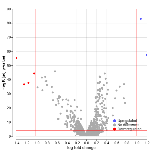
The most upregulated genes in the plot are toward the right (in blue), while the most downregulated genes are toward the left (in red). Other genes with a small magnitude of change are colored in gray. The most statistically significant genes are toward the top of the plot.
You can also export the results of the differential expression analysis in a CSV format. Read more in the Export to CSV section.
Compare a selected cell set between samples/groups
With this differential expression analysis, you can find differentially expressed genes between two experimental groups and plot the respective volcano plot. This analysis uses a pseudobulk limma-voom workflow.
To perform this differential expression analysis and plot the volcano plot go to the Differential expression control. Then choose a cell set you want to compare in the first drop-down menu (1). Choose the first sample/group to compare in the second drop-down menu (2). Lastly, select the second sample/group you want to compare with the first sample/group or choose the option ‘Rest of Samples’ or ‘All other cells’ (3).

When you have made your selections, click compute.

The volcano plot based on the computed differential expression analysis will appear in the plot tile.

The most upregulated genes in the plot are toward the right (in blue), while the most downregulated genes are toward the left (in red). Other genes with a small magnitude of change are colored in gray. The most statistically significant genes are toward the top of the plot.
You can also export the results of the differential expression analysis in a CSV format. Read more in the Export to CSV section.
Export to CSV
When you have performed the differential expression analysis, alongside the volcano plot an ‘Export to CSV’ button is going to appear at the top of the plot window.

Click on the button, and your differential expression results will be automatically downloaded in a CSV file.
Data thresholding
Under the Data thresholding control, you can modify the significance thresholds and the design of the guidelines.

Significance Thresholds
You can change the -log10 (p-value) threshold on the y-axis. To do this, input a new threshold into the input box. This can change which genes are going to be considered upregulated or downregulated. The equivalent p-value is displayed below the input box. See the example below.

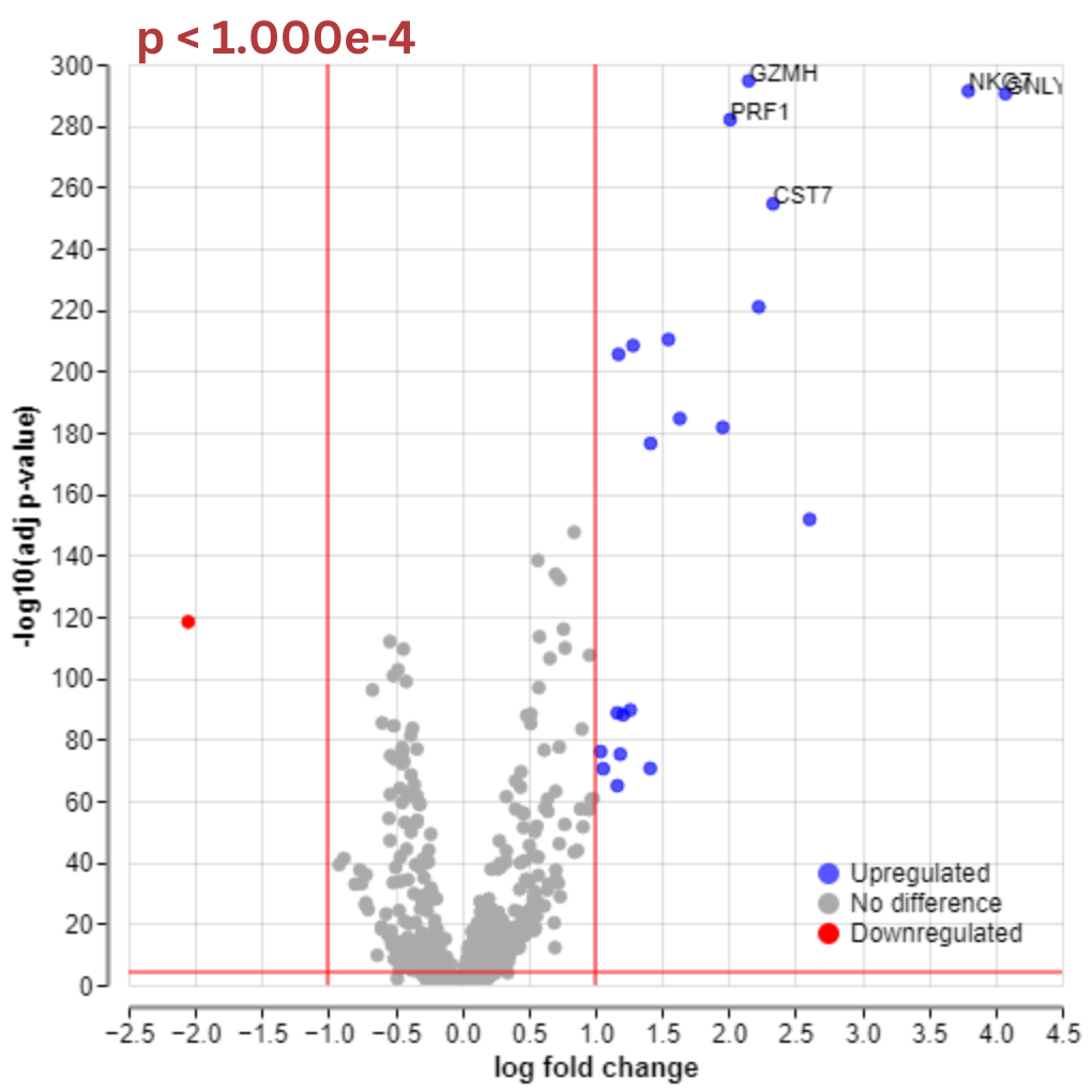


You can also change the fold change (log) value on the x-axis. The fold change is the ratio of gene expression between the two groups being compared. They are then log-transformed. Adjusting the log fold change value threshold can change which genes will be considered upregulated or downregulated. The new value will be represented as the negative and positive log fold change thresholds, as shown in the example below.

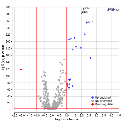


You can also choose to deselect the option ‘Show guideline.’

For both thresholds, deselecting this option will color the guideline black instead of the default red in the plot tile. When you download the plot, the guidelines will disappear completely. See the example below.


Guideline design
Under the guideline design, you can adjust the width and color of the guidelines.
To change the width of the lines, just input the new width value.


You can also change the colors of the guidelines. To do so click on Browse next to “Colors”. Then click on the colored circle on the right of the guideline whose color you want to change.

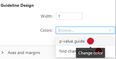
Then simply select a new color. The change is going to be applied automatically. For example, below is a plot with a blue guideline for the p-value.


Colours
Besides color inversion, under the “Colours” control you are able to change the appearance of markers. Click on Browse next to “Markers”. To change the color of gene markers, click on the colored circle on the right of the marker type.


Then choose a new color. The change is going to be applied automatically. In the example below, downregulated genes are now colored purple.


Comparing fewer than 3 samples
Note that for some selections, a warning message will appear:

The message explains that there are fewer than 3 samples with the minimum number of cells required to perform the differential expression calculation in your selected comparison. The most likely explanation is that you are comparing 1 sample to 1 other sample. An alternative explanation is that you are comparing 3 or more samples but that there are too few cells (<10) in one or more of the comparison groups, resulting in only 2 ‘valid’ comparison groups that contain enough cells to perform the calculation.
As the warning message explains, for a comparison between only two ‘valid’ samples it is not possible to compute the differential expression and obtain statistically meaningful results. For such a comparison it is therefore not possible to create a volcano plot in Cellenics®.
In this case, you can still perform the differential expression calculation, but the results will only consist of DE genes and logFC values and should be interpreted with caution and only used for exploratory purposes. No adjusted p-value will be calculated, which means that you will not be able to plot a volcano plot. The plot will look like the image below. However, you can download your results in a CSV format.

Batch Differential Expression Table
Here you can perform DE analysis and download batch DE tables. There are three comparison options.

Generate a full list of marker genes for all cell sets
First, you can download a full list of marker genes for all cell sets, where each cell set will be compared to all other cells, using all samples. You can select which cell sets you want to use for analysis.

When you have selected the cell sets for which marker genes are to be computed in batch, click “Compute and Download”.

A DE table will be created for each cell set.


Compare two selected samples/groups within a cell set for all cell sets
You can also compare two selected samples/groups within a cell set in a batch for all cell sets.
Choose a sample/group you want to compare in the first drop-down menu. (1). Choose another sample/group, or the option ‘Rest of Samples’ or ‘All other cells’ in the second drop-down menu (2). Lastly, select the cell sets within which you want to compare samples/groups (3).

Then click “Compute and Download”. Note that a warning may appear if one or more of the selected samples/groups does not contain enough cells in the selected cell set. In this scenario, comparisons for those samples/groups will be skipped.

Compare between two cell sets for all samples/groups
And lastly, you compare two cell sets for all samples/groups.
Choose a cell set you want to compare in the first drop-down menu. (1). Choose another cell set, or the option ‘Rest of Louvain clusters’ or ‘All other cells’ in the second drop-down menu (2). Lastly, select the sample/group for which you want to batch compare cell sets (3).

Then click “Compute and Download”. Note that you might get a warning message.

The message explains that there are fewer than 3 samples with the minimum number of cells required to perform the differential expression calculation in your selected comparison. The most likely explanation is that you are comparing 1 sample to 1 other sample. An alternative explanation is that you are comparing 3 or more samples but that there are too few cells (<10) in one or more of the comparison groups, resulting in only 2 ‘valid’ comparison groups that contain enough cells to perform the calculation.
As the warning message explains, for a comparison between only two ‘valid’ samples it is not possible to compute the differential expression and obtain statistically meaningful results. For such a comparison it is therefore not possible to create a volcano plot in Cellenics®.
In this case, you can still perform the differential expression calculation, but the results will only consist of DE genes and logFC values and should be interpreted with caution and only used for exploratory purposes. No adjusted p-value will be calculated.
Downloading plots
You can download the plots by clicking on the button with three dots in the top right corner of the plot.

You can save your plots as PNG or SVG. Click on your preferred option to start the download.

You can also download your plot using right-click “Save image as.”
Frequently asked questions
-
The Biomage-hosted community instance of Cellenics® is completely free for academic researchers with small and medium sized datasets of up to 500k cells. When you sign up, please use your academic email address. If you’re looking to become an industry partner, please visit our single cell RNA-seq support service page.
-
We suggest including the following statement in your Methods section: "The single cell RNA-seq dataset was processed, explored and visualised using Cellenics® community instance (https://scp.biomage.net/) hosted by Biomage (https://biomage.net/)."
We recommend that you report the processing settings (filtering thresholds, integration method, etc.) that are available for you to download via the 'Download' button in the Data Management module. We can assist with writing this paragraph, if needed. We can also provide the platform version number - just get in touch with us!
And do keep us up-to-date with your submission and publication - we’d be delighted to hear about (and promote!) your paper!
-
Post your questions, feedback and feature requests on the Biomage community forum for Cellenics® users: https://community.biomage.net
-
Cellenics® is, for the most-part, based on Seurat - a state-of-the-art R toolkit for single cell genomics that is developed and maintained by the Satija lab at the New York Genome Centre. In addition, Cellenics® has added functionality with another powerful R toolkit, namely the Bionconductor SCE (SingleCellExperiment) framework. Throughout Cellenics®, you will find tooltips explanations for each data processing step and statistical analysis process.
But you don't have to take our word for it! Since all the Cellenics® code is open source, you can explore it for yourself on GitHub.
-
We are really excited to hear your feedback! Please use the ‘Feedback’ button at the top of the page in Cellenics®. Alternatively, you can post your feedback on the Biomage community forum for Cellenics® users: https://community.biomage.net