
Single-cell analysis overview by Prof. Peter Kharchenko
Prof. Peter Kharchenko is an internationally renowned Professor of Bioinformatics and a worldwide leader in the field of data analytics. Peter’s lab is now situated at Altos Labs, a new biotechnology company dedicated to unraveling the deep biology of cellular rejuvenation programming. Prof. Peter Kharchenko is also the scientific co-founder of Biomage.
This blog post is an excerpt from Prof. Peter Kharchenko's talk at one of the Cellenics® workshops provided by the Biomage team (see events page). Below this post, you will find the full talk.
In his presentation, Prof. Peter Kharchenko gives an overview of single-cell transcriptomics analysis, a powerful method that has progressed rapidly in recent years. He discusses the growth of single-cell RNA sequencing (scRNA-seq), and the subsequent high data volume. He also considers different single-cell RNA-seq data processing tools, why they are needed, and what cons they have.
Find out about upcoming workshops at https://www.biomage.net/upcoming-events.
Growth of scRNA-seq
Single-cell RNA-seq in particular has been the assay that has progressed rapidly over the past 10 years or so. Here is a plot comparing it with progress in processors (Figure 1). So, we have either in black the number of transistors per CPU on a log10 scale or in red the number of cells in different published studies. And you can see that you have exponential growth in terms of the number of cells.
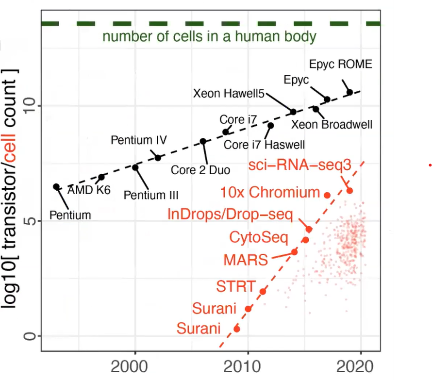
Figure 1. Beating Moore’s law. The number of cells measured by landmark scRNA-seq datasets (red), compared with the increase in the CPU transistor counts (black) over time. Small red dots represent the set of all published scRNA-seq studies. The estimated number of cells in a human body is shown by a green dashed line. Kharchenko, P.V. The triumphs and limitations of computational methods for scRNA-seq. https://doi.org/10.1038/s41592-021-01171-x.
So on one hand, it gives you the capability to observe more cells and find smaller subpopulations, perhaps resolving more subtle differences within the subpopulations. On the other hand, it’s more complicated to analyze as the number of cells reaching the number of transistors means the process doesn’t keep up as well. There's a high data volume, effectively. (...) And you need computation methods and resources to take care of it.
A lot of computations to dispute questions have not been answered well. But there are a lot of methods available. And so, the aim, the initial idea of Cellenics® was to provide this in a cloud environment where you don't have to install everything, and you have user-friendly access to at least core processing elements.
Data processing essentials
So, here (…) on the bottom, you have different tools, and some of these are integrated into Cellenics® (Figure 2). And I'm going to try to emphasize just the basic idea of why they are needed, and then also some of the potential limitations or trade-offs that they make.

Figure 2. Diagram of key preprocessing steps involved in the analysis of scRNA-seq datasets, along with the relevant software tools. Kharchenko, P.V. The triumphs and limitations of computational methods for scRNA-seq. https://doi.org/10.1038/s41592-021-01171-x.
Alignment and molecular counting
So, you have to start with alignment, embargoed, and molecule counting (Figure 2; Alignment and Molecular Counting). And on the surface, it seems like a simple thing. You take a look at the sequence read and one part of it will be mapped to a genome. That's a traditional alignment problem. But the other part will contain barcodes. A cell barcode tells us the identity of the cell from which the read came. And also an incorporated unique molecular identifier (UMI) that allows us to reduce the impact of PCR duplicates.
So it seems like a simple problem, you read the barcode, and you assign the molecule to that cell. If you have already seen a molecule with the same unique molecular identifier, you simply don't count it again. It's still the same molecule. But in reality, things are not that clean. Sequencers make errors. And library synthesis creates errors. And so the alignment and counting routines have to take that into consideration.
So, for instance, a common technique is to keep track of all the barcodes that, let's say, differ by one letter, and then collapse them to the most popular one. If you have a connected graph you count all of this as a single molecule still, because you admit that there could have been single nucleotide mistakes. But of course, you can have two nucleotide mistakes. And that can lead to over-counting, you can have more significant errors (...).
Cell filtering
The other thing, especially in droplet techniques, is that you have a lot of background noise. So, not every droplet that flows through the system will have a cell in it, and the empty droplets, for instance, will have some ambient RNA from the cell suspension incorporated into them. And they get amplified. And it creates a sort of a weak barcode that has relatively few molecules to it. And so they have to be filtered out (Figure 2; Cell Filtering/QC).
But it's a continuum, right? So you have, let's say, some droplets that incorporate maybe cell debris, or comet effects that catch a tail of a cell that's leaking. And that will kind of look like a cell, but not quite. So, typically, these methods have to draw a line somewhere. Here, we just do this by the cell size. So the total number of molecules in the cell, and we rank the cells by it and we look for this type of inflection point.
Assumptions in doublet scoring
So these methods typically try to simulate what this type of pure average replicate would be and then try to eliminate them. And the intuition behind this is that if you have, let's say, actual states of red and green (Figure 2; Doublet Scoring). So, if there are two distinct states, then in biology, you should never get a state that is a pure linear combination of the two, right? So there should be some kind of curvature always if it's a real process. That's the assumption they make.
If you play around with these methods, you'll see very quickly that they're making guesses. And there are a lot of ways of getting different results with them. So first of all, parameters are based on some assumptions. More importantly, if you, for instance, throw out all the blue population (emit it) and rerun the doublet scoring, you'll probably pick up a different set of doublets, if you're running it on a subset of a data set (Figure 2; Doublet Scoring). Those are the unfortunate limitations, and it is just important to be aware of it that none of this is set in stone. These are tools that are based on assumptions and you ideally should keep track of those assumptions.
Secondary analysis
A clean count matrix (Figure 2; Cell Size Estimation) typically serves as the beginning of this secondary analysis. And then, what people try to do is, effectively estimate the structure of these populations in different ways (Figure 3).

Figure 3. Diagram of major steps involved in the analysis of scRNA-seq datasets, along with the relevant software tools. Kharchenko, P.V. The triumphs and limitations of computational methods for scRNA-seq. https://doi.org/10.1038/s41592-021-01171-x.
Cluster analysis
And this is where packages such as Seurat, scanpy, and so on, are particularly useful. This is where they work. And the reason you try to estimate structure is that you're interested in the subpopulations that exist. Clusters, for instance, are probably the most common way of describing the structure of these datasets(Figure 3; Clustering). You have two clusters, three clusters, but it's a crude approximation.
Trajectory analysis
So, you may have a continuous trajectory. And then clusters are not very good at describing and capturing the structure of these populations. We can draw these trajectories(Figure 3; Trajectories). But again, if you pick a different subset of cells, or even if you ask these methods to connect something that is not related by the continuous process via trajectory, they will do it. It's just a computational exercise. But it gives you a way of approximating the structure.
Manifold representation
Most of these methods use this neighbor graph representation of the structure of these populations (Figure 3; Manifold Representation). So, this expression manifold is typically approximated as a neighbor graph. It's flexible enough, and on that neighbor graph, you could do either trajectory fitting or clustering or any other type of estimation.
Dimensionality reduction
To get this neighbor graph effectively, we need to find the closest neighbors for each cell. But to get it, we need to typically move to reduce representation to some kind of medium-dimensional space (Figure 3; Reduction to a medium-dimensional space). Because one of the key issues with this type of genomics is that the overall space is very large, you have 10s of 1000s of genes, (…), and it's just such a high dimensional space that you can’t effectively measure distances in it. So you have to reduce it to some small number of dimensions in order for traditional distances, such as Euclidean distance or correlation, similarity measure to start to work.
Data analysis using Cellenics®
Biomage host a community instance of Cellenics® (available at https://scp.biomage.net/) that’s free for academic users. Cellenics® was developed by © 2020-2022 President and Fellows of Harvard College under the scientific supervision of Prof. Peter Kharchenko and the administrative supervision of the Department of Biomedical Informatics at Harvard Medical School. This software is fast and user-friendly, so biologists don't need prior programming experience to analyze single-cell data.
So, which steps of scRNA-seq data processing are covered in Cellenics®?
The Cellenics® tool provides an in-depth data processing and quality control workflow for raw count matrices (barcodes.tsv/features.tsv/matrix.mtx). This step-by-step workflow filters out empty droplets, dead cells, poor quality cells, and doublets using a classifier, cell size distribution, mitochondrial content, doublet, and a number of genes versus UMIs filters. For example, the Cell size distribution filter has a plot similar to the one in Figure 2 (Cell Filtering/QC). Data are filtered per sample basis within each filter.
The quality control workflow also removes batch effects and reduces the dimensionality of the data. With Cellenics®, you can perform data integration quickly using MNN, Harmony, or Seurat v4. Integrated data is further reduced into a 2-dimensional embedding and visualized by UMAP and t-SNE projection.
Trajectory analysis is also available to determine the structures of populations on a continuous trajectory!
Learn more about the Data Processing features available in Cellenics® here: https://www.biomage.net/user-guide
Full Talk: Single-cell analysis overview by Prof. Peter Kharchenko
Disclaimer:
The talk is transcribed clean verbatim with corrections for readability.